本文通过迁移学习将训练好的VGG16模型应用到图像的多标签分类问题中。该项目数据来自于Kaggle,每张图片可同时属于多个标签。模型的准确度使用F score进行量化,如下表所示:
| 标签 | 预测为Positive(1) | 预测为Negative(0) |
|---|---|---|
| 真值为Positive(1) | TP | FN |
| 真值为Negative(0) | FP | TN |
例如真实标签是(1,0,1,1,0,0), 预测标签是(1,1,0,1,1,0), 则TP=2, FN=1, FP=2, TN=1。$$Precision=frac{TP}{TP+FP}, ext{ }Recall=frac{TP}{TP+FN}, ext{ }F{\_}score=frac{(1+eta^2)*Presicion*Recall}{Recall+eta^2*Precision}$$其中$eta$越小,F score中Precision的权重越大,$eta$等于0时F score就变为Precision;$eta$越大,F score中Recall的权重越大,$eta$趋于无穷大时F score就变为Recall。可以在Keras中自定义该函数(y_pred表示预测概率):
from tensorflow.keras import backend

# calculate fbeta score for multi-label classification
def fbeta(y_true, y_pred, beta=2):
    # clip predictions
    y_pred = backend.clip(y_pred, 0, 1)
    # calculate elements for each sample
    tp = backend.sum(backend.round(backend.clip(y_true * y_pred, 0, 1)), axis=1)
    fp = backend.sum(backend.round(backend.clip(y_pred - y_true, 0, 1)), axis=1)
    fn = backend.sum(backend.round(backend.clip(y_true - y_pred, 0, 1)), axis=1)
    # calculate precision
    p = tp / (tp + fp + backend.epsilon())
    # calculate recall
    r = tp / (tp + fn + backend.epsilon())
    # calculate fbeta, averaged across samples
    bb = beta ** 2
    fbeta_score = backend.mean((1 + bb) * (p * r) / (bb * p + r + backend.epsilon()))
    return fbeta_score
此外在损失函数的使用上多标签分类和多类别(multi-class)分类也有区别,多标签分类使用binary_crossentropy,假设一个样本的真实标签是(1,0,1,1,0,0),预测概率是(0.2, 0.3, 0.4, 0.7, 0.9, 0.2): $$binary{\_}crossentropy ext{ }loss=-(ln 0.2 + ln 0.7 + ln 0.4 + ln 0.7 + ln 0.1 + ln 0.8)/6=0.96$$另外多标签分类输出层的激活函数选择sigmoid而非softmax。模型架构如下所示:
from tensorflow.keras.layers import Dense, Flatten
from tensorflow.keras.optimizers import Adam
from tensorflow.keras.applications.vgg16 import VGG16
from tensorflow.keras.models import Model

def define_model(in_shape=(128, 128, 3), out_shape=17):
    # load model
    base_model = VGG16(weights='imagenet', include_top=False, input_shape=in_shape)
    # mark loaded layers as not trainable
    for layer in base_model.layers: layer.trainable = False
    # make the last block trainable
    tune_layers = [layer.name for layer in base_model.layers if layer.name.startswith('block5_')]
    for layer_name in tune_layers: base_model.get_layer(layer_name).trainable = True
    # add new classifier layers
    flat1  = Flatten()(base_model.layers[-1].output)
    class1 = Dense(128, activation='relu', kernel_initializer='he_uniform')(flat1)
    output = Dense(out_shape, activation='sigmoid')(class1)
    # define new model
    model = Model(inputs=base_model.input, outputs=output)
    # compile model
    opt = Adam(learning_rate=1e-3)
    model.compile(optimizer=opt, loss='binary_crossentropy', metrics=[fbeta])
    model.summary()
    return model
从Kaggle网站上下载数据并解压,将其处理成可被模型读取的数据格式


from os import listdir
from numpy import zeros, asarray, savez_compressed
from pandas import read_csv
from tensorflow.keras.preprocessing.image import load_img, img_to_array

# create a mapping of tags to integers given the loaded mapping file
def create_tag_mapping(mapping_csv):
    labels = set() # create a set of all known tags
    for i in range(len(mapping_csv)):
        tags = mapping_csv['tags'][i].split(' ') # convert spaced separated tags into an array of tags
        labels.update(tags) # add tags to the set of known labels
    labels = sorted(list(labels)) # convert set of labels to a sorted list
    # dict that maps labels to integers, and the reverse
    labels_map = {labels[i]:i for i in range(len(labels))}
    inv_labels_map = {i:labels[i] for i in range(len(labels))}
    return labels_map, inv_labels_map

# create a mapping of filename to a list of tags
def create_file_mapping(mapping_csv):
    mapping = dict()
    for i in range(len(mapping_csv)):
        name, tags = mapping_csv['image_name'][i], mapping_csv['tags'][i]
        mapping[name] = tags.split(' ')
    return mapping

# create a one hot encoding for one list of tags
def one_hot_encode(tags, mapping):
    encoding = zeros(len(mapping), dtype='uint8') # create empty vector
    # mark 1 for each tag in the vector
    for tag in tags: encoding[mapping[tag]] = 1
    return encoding

# load all images into memory
def load_dataset(path, file_mapping, tag_mapping):
    photos, targets = list(), list()
    # enumerate files in the directory
    for filename in listdir(path):
        photo = load_img(path + filename, target_size=(128,128)) # load image
        photo = img_to_array(photo, dtype='uint8') # convert to numpy array
        tags = file_mapping[filename[:-4]] # get tags
        target = one_hot_encode(tags, tag_mapping) # one hot encode tags
        photos.append(photo)
        targets.append(target)
    X = asarray(photos, dtype='uint8')
    y = asarray(targets, dtype='uint8')
    return X, y

filename = 'train_v2.csv' # load the target file
mapping_csv = read_csv(filename)
tag_mapping, _ = create_tag_mapping(mapping_csv) # create a mapping of tags to integers
file_mapping = create_file_mapping(mapping_csv) # create a mapping of filenames to tag lists
folder = 'train-jpg/' # load the jpeg images
X, y = load_dataset(folder, file_mapping, tag_mapping)
print(X.shape, y.shape)
savez_compressed('planet_data.npz', X, y) # save both arrays to one file in compressed format
接下来再建立两个辅助函数,第一个函数用来分割训练集和验证集,第二个函数用来画出模型在训练过程中的学习曲线
import numpy as np
from matplotlib import pyplot
from sklearn.model_selection import train_test_split

# load train and test dataset
def load_dataset():
    # load dataset
    data = np.load('planet_data.npz')
    X, y = data['arr_0'], data['arr_1']
    # separate into train and test datasets
    trainX, testX, trainY, testY = train_test_split(X, y, test_size=0.3, random_state=1)
    print(trainX.shape, trainY.shape, testX.shape, testY.shape)
    return trainX, trainY, testX, testY

# plot diagnostic learning curves
def summarize_diagnostics(history):
    # plot loss
    pyplot.subplot(121)
    pyplot.title('Cross Entropy Loss')
    pyplot.plot(history.history['loss'], color='blue', label='train')
    pyplot.plot(history.history['val_loss'], color='orange', label='test')
    # plot accuracy
    pyplot.subplot(122)
    pyplot.title('Fbeta')
    pyplot.plot(history.history['fbeta'], color='blue', label='train')
    pyplot.plot(history.history['val_fbeta'], color='orange', label='test')
    pyplot.show()
使用数据扩充技术(Data Augmentation)对模型进行训练
from tensorflow.keras.preprocessing.image import ImageDataGenerator
from tensorflow.keras.applications.vgg16 import preprocess_input
from tensorflow.keras.callbacks import ModelCheckpoint

trainX, trainY, testX, testY = load_dataset() # load dataset
# create data generator using augmentation
# vertical flip is reasonable since the pictures are satellite images
train_datagen = ImageDataGenerator(horizontal_flip=True, vertical_flip=True, rotation_range=90, preprocessing_function=preprocess_input)
test_datagen = ImageDataGenerator(preprocessing_function=preprocess_input)
# prepare generators
train_it = train_datagen.flow(trainX, trainY, batch_size=128)
test_it = test_datagen.flow(testX, testY, batch_size=128)
# define model
model = define_model()
# fit model
# When one epoch ends, the validation generator will yield validation_steps batches, then average the evaluation results of all batches
checkpointer = ModelCheckpoint(filepath='./weights.best.vgg16.hdf5', verbose=1, save_best_only=True)
history = model.fit_generator(train_it, steps_per_epoch=len(train_it), validation_data=test_it, validation_steps=len(test_it),
                              epochs=15, callbacks=[checkpointer], verbose=0)
# evaluate optimal model
# For simplicity, the validation set is used to test the model here. In fact an entirely new test set should have been used.
model.load_weights('./weights.best.vgg16.hdf5') #load stored optimal coefficients
loss, fbeta = model.evaluate_generator(test_it, steps=len(test_it), verbose=0)
print('> loss=%.3f, fbeta=%.3f' % (loss, fbeta)) # loss=0.108, fbeta=0.884
model.save('final_model.h5')
# learning curves
summarize_diagnostics(history)
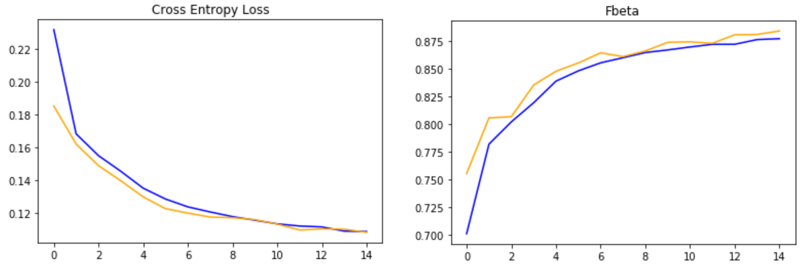
蓝线代表训练集,黄线代表验证集