一 数据格式
1.1 dicom
DICOM是医学图像中标准文件,这些文件包含了诸多的元数据信息(比如像素尺寸,每个维度的一像素代表真实世界里的长度)。此处以kaggle Data Science Bowl 数据集为例。
data-science-bowl-2017。数据列表如下:
后缀为 .dcm。
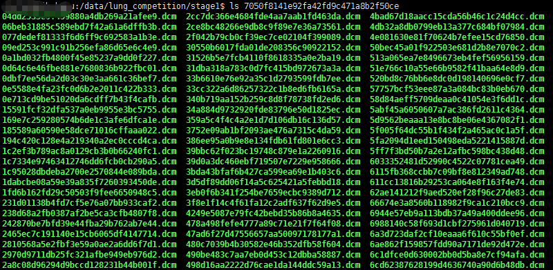
每个病人的一次扫描CT(scan)可能有几十到一百多个dcm数据文件(slices)。可以使用 python的dicom包读取,读取示例代码如下:
dicom.read_file('/data/lung_competition/stage1/7050f8141e92fa42fd9c471a8b2f50ce/498d16aa2222d76cae1da144ddc59a13.dcm')
其pixl_array包含了真实数据。
slices =[dicom.read_file(os.path.join(folder_name,filename))for filename in os.listdir(folder_name)]slices = np.stack([s.pixel_array for s in slices])
1.2 mhd格式
mhd格式是另外一种数据格式,来源于(LUNA2016)[https://luna16.grand-challenge.org/data/]。每个病人一个mhd文件和一个同名的raw文件。如下:
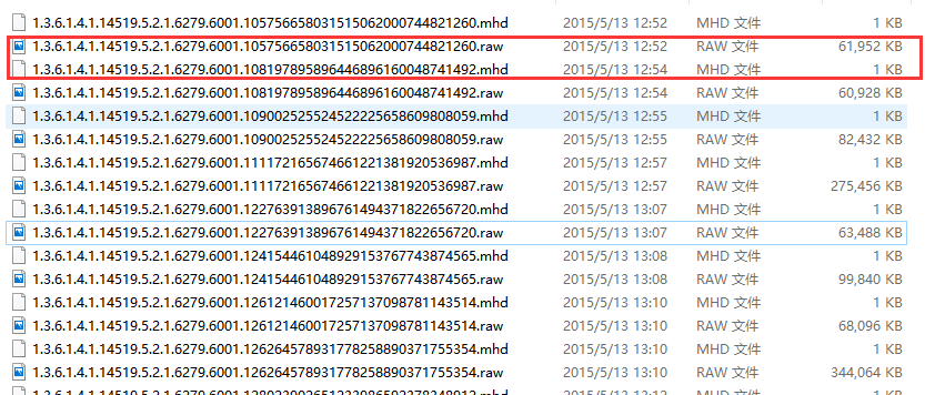
一个mhd通常有几百兆,对应的raw文件只有1kb。mhd文件需要借助python的SimpleITK包来处理。SimpleITK 示例代码如下:
importSimpleITKas sitkitk_img = sitk.ReadImage(img_file)img_array = sitk.GetArrayFromImage(itk_img)# indexes are z,y,x (notice the ordering)num_z, height, width = img_array.shape #heightXwidth constitute the transverse planeorigin = np.array(itk_img.GetOrigin())# x,y,z Origin in world coordinates (mm)spacing = np.array(itk_img.GetSpacing())# spacing of voxels in world coor. (mm)
需要注意的是,SimpleITK的img_array的数组不是直接的像素值,而是相对于CT扫描中原点位置的差值,需要做进一步转换。转换步骤参考 SimpleITK图像转换
1.3 查看CT扫描文件软件
一个开源免费的查看软件 mango
二 dicom格式数据处理过程
2.1 处理思路
首先,需要明白的是医学扫描图像(scan)其实是三维图像,使用代码读取之后开源查看不同的切面的切片(slices),可以从不同轴切割
如下图展示了一个病人CT扫描图中,其中部分切片slices
其次,CT扫描图是包含了所有组织的,如果直接去看,看不到任何有用信息。需要做一些预处理,预处理中一个重要的概念是放射剂量,衡量单位为HU(Hounsfield Unit),下表是不同放射剂量对应的组织器官
| substance | HU |
|---|---|
| 空气 | -1000 |
| 肺 | -500 |
| 脂肪 | -100到-50 |
| 水 | 0 |
| CSF | 15 |
| 肾 | 30 |
| 血液 | +30到+45 |
| 肌肉 | +10到+40 |
| 灰质 | +37到+45 |
| 白质 | +20到+30 |
| Liver | +40到+60 |
| 软组织,constrast | +100到+300 |
| 骨头 | +700(软质骨)到+3000(皮质骨) |
HounsfieldUnit= pixel_value * rescale_slope + rescale_intercept
一般情况rescale slope = 1, intercept = -1024。
上表中肺部组织的HU数值为-500,但通常是大于这个值,比如-320、-400。挑选出这些区域,然后做其他变换抽取出肺部像素点。
2.2 先载入必要的包
# -*- coding:utf-8 -*-'''this script is used for basic process of lung 2017 in Data Science Bowl'''import globimport osimport pandas as pdimportSimpleITKas sitkimport numpy as np # linear algebraimport pandas as pd # data processing, CSV file I/O (e.g. pd.read_csv)import skimage, osfrom skimage.morphology import ball, disk, dilation, binary_erosion, remove_small_objects, erosion, closing, reconstruction, binary_closingfrom skimage.measure import label,regionprops, perimeterfrom skimage.morphology import binary_dilation, binary_openingfrom skimage.filters import roberts, sobelfrom skimage import measure, featurefrom skimage.segmentation import clear_borderfrom skimage import datafrom scipy import ndimage as ndiimport matplotlib#matplotlib.use('Agg')import matplotlib.pyplot as pltfrom mpl_toolkits.mplot3d.art3d importPoly3DCollectionimport dicomimport scipy.miscimport numpy as np
如下代码是载入一个扫描面,包含了多个切片(slices),我们仅简化的将其存储为python列表。数据集中每个目录都是一个扫描面集(一个病人)。有个元数据域丢失,即Z轴方向上的像素尺寸,也即切片的厚度 。所幸,我们可以用其他值推测出来,并加入到元数据中。
# Load the scans in given folder pathdef load_scan(path):slices =[dicom.read_file(path +'/'+ s)for s in os.listdir(path)]slices.sort(key =lambda x:int(x.ImagePositionPatient[2]))try:slice_thickness = np.abs(slices[0].ImagePositionPatient[2]- slices[1].ImagePositionPatient[2])except:slice_thickness = np.abs(slices[0].SliceLocation- slices[1].SliceLocation)for s in slices:s.SliceThickness= slice_thicknessreturn slices
2.3 灰度值转换为HU单元
首先去除灰度值为 -2000的pixl_array,CT扫描边界之外的灰度值固定为-2000(dicom和mhd都是这个值)。第一步是设定这些值为0,当前对应为空气(值为0)
回到HU单元,乘以rescale比率并加上intercept(存储在扫描面的元数据中)。
def get_pixels_hu(slices):image = np.stack([s.pixel_array for s in slices])# Convert to int16 (from sometimes int16),# should be possible as values should always be low enough (<32k)image = image.astype(np.int16)# Set outside-of-scan pixels to 0# The intercept is usually -1024, so air is approximately 0image[image ==-2000]=0# Convert to Hounsfield units (HU)for slice_number in range(len(slices)):intercept = slices[slice_number].RescaleInterceptslope = slices[slice_number].RescaleSlopeif slope !=1:image[slice_number]= slope * image[slice_number].astype(np.float64)image[slice_number]= image[slice_number].astype(np.int16)image[slice_number]+= np.int16(intercept)return np.array(image, dtype=np.int16)
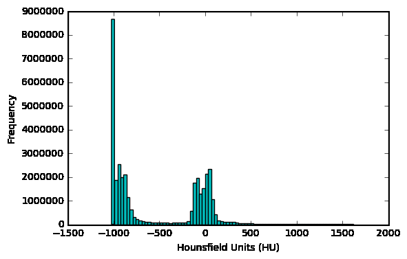
可以查看病人的扫描HU值分布情况
first_patient = load_scan(INPUT_FOLDER + patients[0])first_patient_pixels = get_pixels_hu(first_patient)plt.hist(first_patient_pixels.flatten(), bins=80, color='c')plt.xlabel("Hounsfield Units (HU)")plt.ylabel("Frequency")plt.show()
2.4 重采样
不同扫描面的像素尺寸、粗细粒度是不同的。这不利于我们进行CNN任务,我们可以使用同构采样。
一个扫描面的像素区间可能是[2.5,0.5,0.5],即切片之间的距离为2.5mm。可能另外一个扫描面的范围是[1.5,0.725,0.725]。这可能不利于自动分析。
常见的处理方法是从全数据集中以固定的同构分辨率重新采样,将所有的东西采样为1mmx1mmx1mm像素。
def resample(image, scan, new_spacing=[1,1,1]):# Determine current pixel spacingspacing = map(float,([scan[0].SliceThickness]+ scan[0].PixelSpacing))spacing = np.array(list(spacing))resize_factor = spacing / new_spacingnew_real_shape = image.shape * resize_factornew_shape = np.round(new_real_shape)real_resize_factor = new_shape / image.shapenew_spacing = spacing / real_resize_factorimage = scipy.ndimage.interpolation.zoom(image, real_resize_factor, mode='nearest')return image, new_spacing
现在重新取样病人的像素,将其映射到一个同构分辨率 1mm x1mm x1mm。
pix_resampled, spacing = resample(first_patient_pixels, first_patient,[1,1,1])
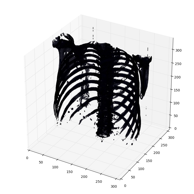
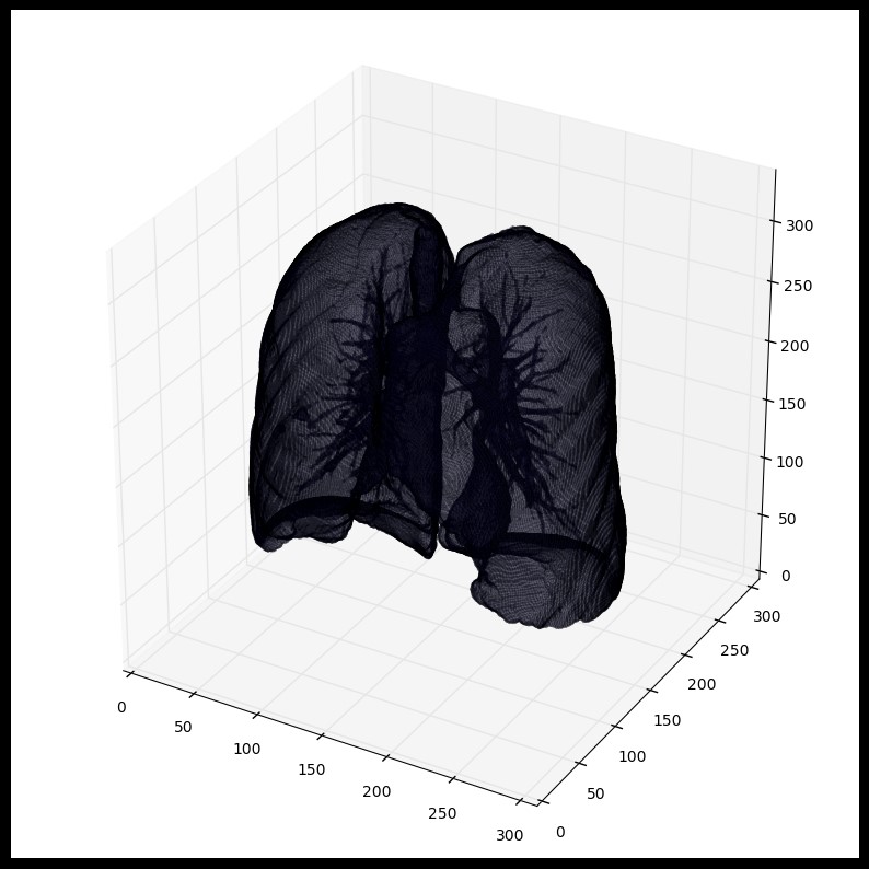
使用matplotlib输出肺部扫描的3D图像方法。可能需要一两分钟。
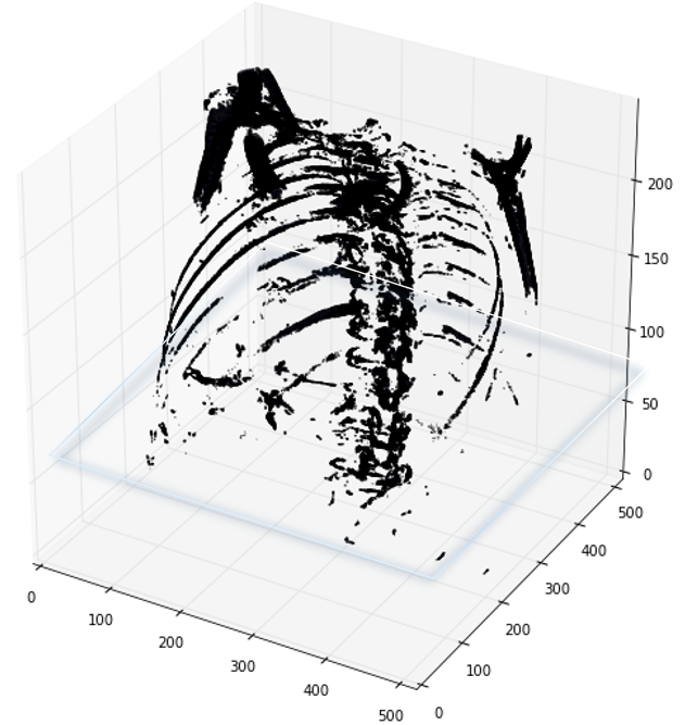
def plot_3d(image, threshold=-300):# Position the scan upright,# so the head of the patient would be at the top facing the camerap = image.transpose(2,1,0)verts, faces = measure.marching_cubes(p, threshold)fig = plt.figure(figsize=(10,10))ax = fig.add_subplot(111, projection='3d')# Fancy indexing: `verts[faces]` to generate a collection of trianglesmesh =Poly3DCollection(verts[faces], alpha=0.1)face_color =[0.5,0.5,1]mesh.set_facecolor(face_color)ax.add_collection3d(mesh)ax.set_xlim(0, p.shape[0])ax.set_ylim(0, p.shape[1])ax.set_zlim(0, p.shape[2])plt.show()
打印函数有个阈值参数,来打印特定的结构,比如tissue或者骨头。400是一个仅仅打印骨头的阈值(HU对照表)
plot_3d(pix_resampled,400)
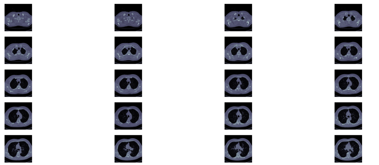
2.5 输出一个病人scans中所有切面slices
def plot_ct_scan(scan):'''plot a few more images of the slices:param scan::return:'''f, plots = plt.subplots(int(scan.shape[0]/20)+1,4, figsize=(50,50))for i in range(0, scan.shape[0],5):plots[int(i /20),int((i %20)/5)].axis('off')plots[int(i /20),int((i %20)/5)].imshow(scan[i], cmap=plt.cm.bone)
此方法的效果示例如下:

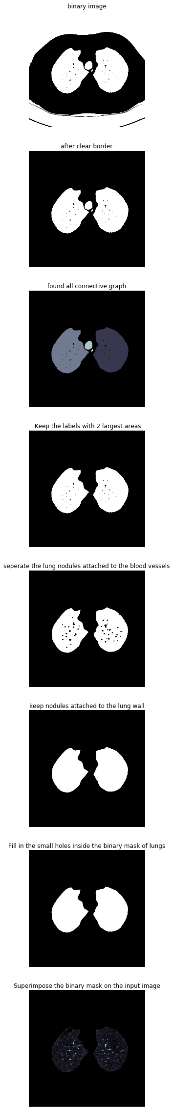
2.6 定义分割出CT切面里面肺部组织的函数
下面的代码使用了pythonde 的图像形态学操作。具体可以参考python高级形态学操作
def get_segmented_lungs(im, plot=False):'''This funtion segments the lungs from the given 2D slice.'''if plot ==True:f, plots = plt.subplots(8,1, figsize=(5,40))'''Step 1: Convert into a binary image.'''binary = im <604if plot ==True:plots[0].axis('off')plots[0].set_title('binary image')plots[0].imshow(binary, cmap=plt.cm.bone)'''Step 2: Remove the blobs connected to the border of the image.'''cleared = clear_border(binary)if plot ==True:plots[1].axis('off')plots[1].set_title('after clear border')plots[1].imshow(cleared, cmap=plt.cm.bone)'''Step 3: Label the image.'''label_image = label(cleared)if plot ==True:plots[2].axis('off')plots[2].set_title('found all connective graph')plots[2].imshow(label_image, cmap=plt.cm.bone)'''Step 4: Keep the labels with 2 largest areas.'''areas =[r.area for r in regionprops(label_image)]areas.sort()if len(areas)>2:for region in regionprops(label_image):if region.area < areas[-2]:for coordinates in region.coords:label_image[coordinates[0], coordinates[1]]=0binary = label_image >0if plot ==True:plots[3].axis('off')plots[3].set_title(' Keep the labels with 2 largest areas')plots[3].imshow(binary, cmap=plt.cm.bone)'''Step 5: Erosion operation with a disk of radius 2. This operation isseperate the lung nodules attached to the blood vessels.'''selem = disk(2)binary = binary_erosion(binary, selem)if plot ==True:plots[4].axis('off')plots[4].set_title('seperate the lung nodules attached to the blood vessels')plots[4].imshow(binary, cmap=plt.cm.bone)'''Step 6: Closure operation with a disk of radius 10. This operation isto keep nodules attached to the lung wall.'''selem = disk(10)binary = binary_closing(binary, selem)if plot ==True:plots[5].axis('off')plots[5].set_title('keep nodules attached to the lung wall')plots[5].imshow(binary, cmap=plt.cm.bone)'''Step 7: Fill in the small holes inside the binary mask of lungs.'''edges = roberts(binary)binary = ndi.binary_fill_holes(edges)if plot ==True:plots[6].axis('off')plots[6].set_title('Fill in the small holes inside the binary mask of lungs')plots[6].imshow(binary, cmap=plt.cm.bone)'''Step 8: Superimpose the binary mask on the input image.'''get_high_vals = binary ==0im[get_high_vals]=0if plot ==True:plots[7].axis('off')plots[7].set_title('Superimpose the binary mask on the input image')plots[7].imshow(im, cmap=plt.cm.bone)return im
此方法每个步骤对图像做不同的处理,依次为二值化、清除边界、连通区域标记、腐蚀操作、闭合运算、孔洞填充、效果如下:
2.7 肺部图像分割
为了减少有问题的空间,我们可以分割肺部图像(有时候是附近的组织)。这包含一些步骤,包括区域增长和形态运算,此时,我们只分析相连组件。
步骤如下:
阈值图像(-320HU是个极佳的阈值,但是此方法中不是必要)
处理相连的组件,以决定当前患者的空气的标签,以1填充这些二值图像
可选:当前扫描的每个轴上的切片,选定最大固态连接的组织(当前患者的肉体和空气),并且其他的为0。以掩码的方式填充肺部结构。
只保留最大的气袋(人类躯体内到处都有气袋)
def largest_label_volume(im, bg=-1):vals, counts = np.unique(im, return_counts=True)counts = counts[vals != bg]vals = vals[vals != bg]if len(counts)>0:return vals[np.argmax(counts)]else:returnNonedef segment_lung_mask(image, fill_lung_structures=True):# not actually binary, but 1 and 2.# 0 is treated as background, which we do not wantbinary_image = np.array(image >-320, dtype=np.int8)+1labels = measure.label(binary_image)# Pick the pixel in the very corner to determine which label is air.# Improvement: Pick multiple background labels from around the patient# More resistant to "trays" on which the patient lays cutting the air# around the person in halfbackground_label = labels[0,0,0]#Fill the air around the personbinary_image[background_label == labels]=2# Method of filling the lung structures (that is superior to something like# morphological closing)if fill_lung_structures:# For every slice we determine the largest solid structurefor i, axial_slice in enumerate(binary_image):axial_slice = axial_slice -1labeling = measure.label(axial_slice)l_max = largest_label_volume(labeling, bg=0)if l_max isnotNone:#This slice contains some lungbinary_image[i][labeling != l_max]=1binary_image -=1#Make the image actual binarybinary_image =1-binary_image # Invert it, lungs are now 1# Remove other air pockets insided bodylabels = measure.label(binary_image, background=0)l_max = largest_label_volume(labels, bg=0)if l_max isnotNone:# There are air pocketsbinary_image[labels != l_max]=0return binary_image
查看切割效果
segmented_lungs = segment_lung_mask(pix_resampled,False)segmented_lungs_fill = segment_lung_mask(pix_resampled,True)plot_3d(segmented_lungs,0)
我们可以将肺内的结构也包含进来(结节是固体),不仅仅只是肺部内的空气
plot_3d(segmented_lungs_fill,0)
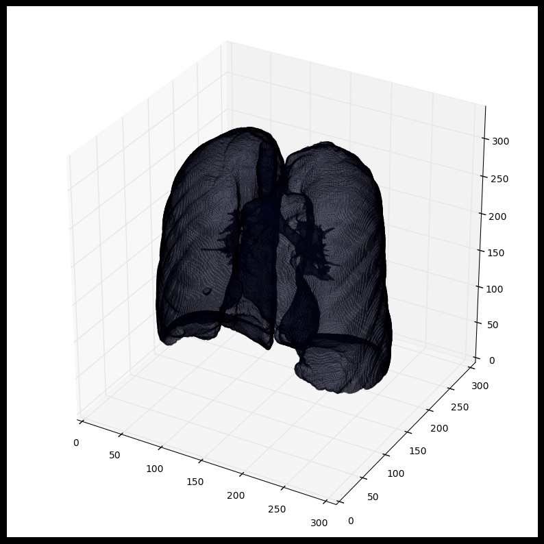
使用mask时,要注意首先进行形态扩充(python的skimage的skimage.morphology)操作(即使用圆形kernel,结节是球体),参考 python形态操作。这会在所有方向(维度)上扩充mask。仅仅肺部的空气+结构将不会包含所有结节,事实上有可能遗漏黏在肺部一侧的结节(这会经常出现,所以建议最好是扩充mask)。
2.8 数据标准化处理
归一化处理
当前的值范围是[-1024,2000]。而任意大于400的值并不是处理肺结节需要考虑,因为它们都是不同反射密度下的骨头。LUNA16竞赛中常用来做归一化处理的阈值集是-1000和400.以下代码
归一化
MIN_BOUND =-1000.0MAX_BOUND =400.0def normalize(image):image =(image - MIN_BOUND)/(MAX_BOUND - MIN_BOUND)image[image>1]=1.image[image<0]=0.return image
0值中心化
简单来说就是所有像素值减去均值。LUNA16竞赛中的均值大约是0.25.
不要对每一张图像做零值中心化(此处像是在kernel中完成的)CT扫描器返回的是校准后的精确HU计量。不会出现普通图像中会出现某些图像低对比度和明亮度的情况
PIXEL_MEAN =0.25def zero_center(image):image = image - PIXEL_MEANreturn image
归一化和零值中心化的操作主要是为了后续训练网络,零值中心化是网络收敛的关键。
三 mhd格式数据处理过程
3.1 处理思路
mhd的数据只是格式与dicom不一样,其实质包含的都是病人扫描。处理MHD需要借助SimpleIKT这个包,处理思路详情可以参考Data Science Bowl2017的toturail Data Science Bowl 2017。需要注意的是MHD格式的数据没有HU值,它的值域范围与dicom很不同。
我们以LUNA2016年的数据处理流程为例。参考代码为 LUNA2016数据切割
3.2 载入必要的包
importSimpleITKas sitkimport numpy as npimport csvfrom glob import globimport pandas as pdfile_list=glob(luna_subset_path+"*.mhd")####################### Helper function to get rows in data frame associated# with each filedef get_filename(case):global file_listfor f in file_list:ifcasein f:return(f)## The locations of the nodesdf_node = pd.read_csv(luna_path+"annotations.csv")df_node["file"]= df_node["seriesuid"].apply(get_filename)df_node = df_node.dropna()####### Looping over the image files#fcount =0for img_file in file_list:print"Getting mask for image file %s"% img_file.replace(luna_subset_path,"")mini_df = df_node[df_node["file"]==img_file]#get all nodules associate with fileif len(mini_df)>0:# some files may not have a nodule--skipping thosebiggest_node = np.argsort(mini_df["diameter_mm"].values)[-1]# just using the biggest nodenode_x = mini_df["coordX"].values[biggest_node]node_y = mini_df["coordY"].values[biggest_node]node_z = mini_df["coordZ"].values[biggest_node]diam = mini_df["diameter_mm"].values[biggest_node]
3.3 LUNA16的MHD格式数据的值
一直在寻找MHD格式数据的处理方法,对于dicom格式的CT有很多论文根据其HU值域可以轻易地分割肺、骨头、血液等,但是对于MHD没有这样的参考。从LUNA16论坛得到的解释是,LUNA16的MHD数据已经转换为HU值了,不需要再使用slope和intercept来做rescale变换了。此论坛主题下,有人提出MHD格式没有提供pixel spacing(mm) 和 slice thickness(mm) ,而标准文件annotation.csv文件中结节的半径和坐标都是mm单位,最后确认的是MHD格式文件中只保留了体素尺寸以及坐标原点位置,没有保存slice thickness。即,dicom才是原始数据格式。
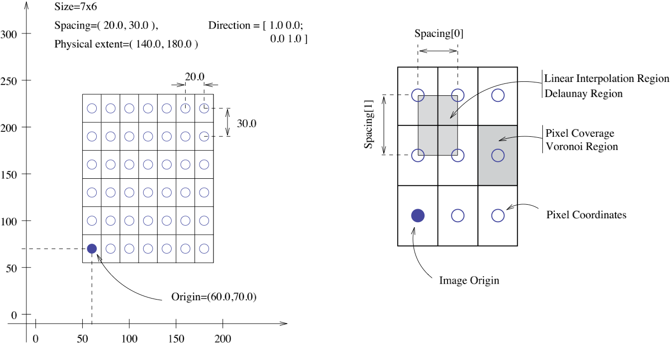
3.4 坐标体系变换
MHD值的坐标体系是体素,以mm为单位(dicom的值是GV灰度值)。结节的位置是CT scanner坐标轴里面相对原点的mm值,需要将其转换到真实坐标轴位置,可以使用SimpleITK包中的 GetOrigin() ` GetSpacing()`。图像数据是以512x512数组的形式给出的。
坐标变换如下:
相应的代码处理如下:
itk_img = sitk.ReadImage(img_file)img_array = sitk.GetArrayFromImage(itk_img)# indexes are z,y,x (notice the ordering)center = np.array([node_x,node_y,node_z])# nodule centerorigin = np.array(itk_img.GetOrigin())# x,y,z Origin in world coordinates (mm)spacing = np.array(itk_img.GetSpacing())# spacing of voxels in world coor. (mm)v_center =np.rint((center-origin)/spacing)# nodule center in voxel space (still x,y,z ordering)
在LUNA16的标注CSV文件中标注了结节中心的X,Y,Z轴坐标,但是实际取值的时候取的是Z轴最后三层的数组(img_array)。
下述代码只提取了包含结节的最后三个slice的数据,代码参考自 LUNA_mask_extraction.py
i =0for i_z in range(int(v_center[2])-1,int(v_center[2])+2):mask = make_mask(center,diam,i_z*spacing[2]+origin[2],width,height,spacing,origin)masks[i]= maskimgs[i]= matrix2int16(img_array[i_z])i+=1np.save(output_path+"images_%d.npy"%(fcount),imgs)np.save(output_path+"masks_%d.npy"%(fcount),masks)
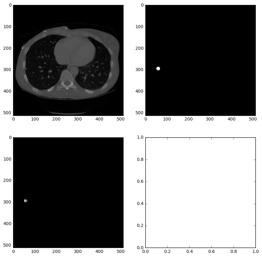
3.5 查看结节
以下代码用于查看原始CT和结节mask。其实就是用matplotlib打印上一步存储的npy文件。
import matplotlib.pyplot as pltimgs = np.load(output_path+'images_0.npy')masks = np.load(output_path+'masks_0.npy')for i in range(len(imgs)):print"image %d"% ifig,ax = plt.subplots(2,2,figsize=[8,8])ax[0,0].imshow(imgs[i],cmap='gray')ax[0,1].imshow(masks[i],cmap='gray')ax[1,0].imshow(imgs[i]*masks[i],cmap='gray')plt.show()raw_input("hit enter to cont : ")
接下来的处理和DICOM格式数据差不多,腐蚀膨胀、连通区域标记等。
参考信息:
灰度值是pixel value经过重重LUT转换得到的用来进行显示的值,而这个转换过程是不可逆的,也就是说,灰度值无法转换为ct值。只能根据窗宽窗位得到一个大概的范围。 pixel value经过modality lut得到Hu,但是怀疑pixelvalue的读取出了问题。dicom文件中存在(0028,0106)(0028,0107)两个tag,分别是最大最小pixel value,可以用来检验你读取的pixel value 矩阵是否正确。
LUT全称look up table,实际上就是一张像素灰度值的映射表,它将实际采样到的像素灰度值经过一定的变换如阈值、反转、二值化、对比度调整、线性变换等,变成了另外一 个与之对应的灰度值,这样可以起到突出图像的有用信息,增强图像的光对比度的作用。