摘要:
深度自编码器(Deep Autoencoder)MATLAB解读深度自编码器首先用受限玻尔兹曼机进行逐层预训练,得到初始的权值与偏置。然后,自编码得到重构数据,通过BP算法进行全局微调权值与偏置。
作者:凯鲁嘎吉 - 博客园http://www.cnblogs.com/kailugaji/
这篇文章主要讲解Hinton在2006年Science上提出的一篇文章“Reducing the dimensionality of data with neural networks”的主要思想与MATLAB程序解读。
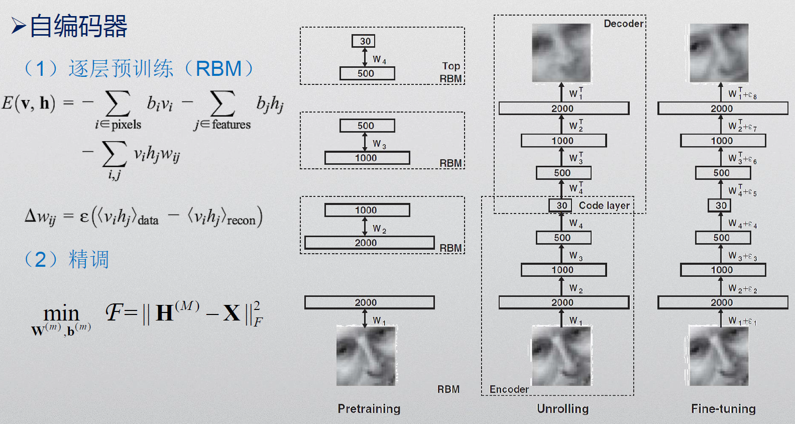
深度自编码器首先用受限玻尔兹曼机进行逐层预训练,得到初始的权值与偏置(权值与偏置的更新过程用对比散度CD-1算法)。然后,自编码得到重构数据,通过BP算法进行全局微调权值与偏置(权值与偏置的更新过程用Polak-Ribiere共轭梯度法)。
1.mnistdeepauto.m
%% 自编码器网络结构:784->1000->500->250->30->250->500->1000->784
clear all
close all
maxepoch=50; %In the Science paper we use maxepoch=50, but it works just fine. 最大迭代数
numhid=1000; numpen=500; numpen2=250; numopen=30;%rbm每层神经元个数1000-500-250-30
%%  数据预处理
%转换数据格式
fprintf(1,'Converting Raw files into Matlab format
');
converter;
%50个来回迭代
fprintf(1,'Pretraining a deep autoencoder.
');
fprintf(1,'The Science paper used 50 epochs. This uses %3i
', maxepoch);
%对数据进行批处理
makebatches;
[numcases numdims numbatches]=size(batchdata);%每批样本数、维度、批数
%%  逐层预训练阶段(用RBM)
%%可见层->1000隐含层
fprintf(1,'Pretraining Layer 1 with RBM: %d-%d
',numdims,numhid);
restart=1;
rbm; %0、1变量 输出权值与偏置的初始更新值
hidrecbiases=hidbiases;
save mnistvh vishid hidrecbiases visbiases;%保存第1个rbm的权值、隐含层偏置项、可视化层偏置项,为mnistvh.mat 784*1000 1*1000 1*784
%%1000隐含层->500隐含层
fprintf(1,'
Pretraining Layer 2 with RBM: %d-%d
',numhid,numpen);
batchdata=batchposhidprobs;
numhid=numpen;
restart=1;
rbm;  %0、1变量 输出权值与偏置的初始更新值
hidpen=vishid; penrecbiases=hidbiases; hidgenbiases=visbiases;
save mnisthp hidpen penrecbiases hidgenbiases;%保存第2个rbm的权值、隐含层偏置项、可视化层偏置项,为mnisthp.mat   1000*500 1*500 1*1000
%%500隐含层->250隐含层
fprintf(1,'
Pretraining Layer 3 with RBM: %d-%d
',numpen,numpen2);
batchdata=batchposhidprobs;
numhid=numpen2;
restart=1;
rbm; %0、1变量 输出权值与偏置的初始更新值
hidpen2=vishid; penrecbiases2=hidbiases; hidgenbiases2=visbiases;
save mnisthp2 hidpen2 penrecbiases2 hidgenbiases2;%保存第3个rbm的权值、隐含层偏置项、可视化层偏置项,为mnisthp2.mat  500*250 1*250 1*500
%250隐含层->30隐含层
fprintf(1,'
Pretraining Layer 4 with RBM: %d-%d
',numpen2,numopen);
batchdata=batchposhidprobs;
numhid=numopen;
restart=1;
rbmhidlinear;  %激活函数为f(x)=x,实值变量 输出权值与偏置的初始更新值
hidtop=vishid; toprecbiases=hidbiases; topgenbiases=visbiases;
save mnistpo hidtop toprecbiases topgenbiases;%保存第4个rbm的权值、隐含层偏置项、可视化层偏置项,为mnistpo.mat  250*30 1*30 1*250
%%  BP全局调参
backprop; %微调权值与偏置
2.converter.m
%%将gz格式转为matlab的文件格式
%实现的功能是将样本集从.ubyte格式转换成.ascii格式,然后继续转换成.mat格式。
% % 作用:把测试数据集和训练数据集转换为.mat格式
% 最终得到的测试数据集:test(0~9).mat
% 最终得到的训练数据集:digit(0~9).mat
% %% 首先转换测试数据集的格式 Work with test files first
fprintf(1,'You first need to download files:
 train-images-idx3-ubyte.gz
 train-labels-idx1-ubyte.gz
 t10k-images-idx3-ubyte.gz
 t10k-labels-idx1-ubyte.gz
 from http://yann.lecun.com/exdb/mnist/
 and gunzip them
');
%该文件前四个32位的数字是数据信息  magic number, number of image, number of rows, number of columns
f = fopen('t10k-images-idx3-ubyte','r');
[a,count] = fread(f,4,'int32');
%该文件前两个32位的数字是数据信息  magic number, number of image
g = fopen('t10k-labels-idx1-ubyte','r');
[l,count] = fread(g,2,'int32');
fprintf(1,'Starting to convert Test MNIST images (prints 10 dots)
');
n = 1000;
%Df中存的是.ascii文件代号
Df = cell(1,10);
for d=0:9,
  Df{d+1} = fopen(['test' num2str(d) '.ascii'],'w');
end;
%一次从测试集(1w)中读入1000个图片和标签  rawlabel 1000*1  rawimages 784*1000
for i=1:10,
  fprintf('.');
  rawimages = fread(f,28*28*n,'uchar');
  rawlabels = fread(g,n,'uchar');
  rawimages = reshape(rawimages,28*28,n);
%在对应文档中输入图片的01值(3个整数位)换行
  for j=1:n,
    fprintf(Df{rawlabels(j)+1},'%3d ',rawimages(:,j));
    fprintf(Df{rawlabels(j)+1},'
');
  end;
end;
fprintf(1,'
');
for d=0:9,
  fclose(Df{d+1});
  D = load(['test' num2str(d) '.ascii'],'-ascii');%读取.ascii 中的数据D=内包含样本数*784
  fprintf('%5d Digits of class %d
',size(D,1),d);
  save(['test' num2str(d) '.mat'],'D','-mat');%转化为.mat文件
end;
% 然后转换训练数据集的格式 Work with trainig files second
f = fopen('train-images-idx3-ubyte','r');
[a,count] = fread(f,4,'int32');
g = fopen('train-labels-idx1-ubyte','r');
[l,count] = fread(g,2,'int32');
fprintf(1,'Starting to convert Training MNIST images (prints 60 dots)
');
n = 1000;
Df = cell(1,10);
for d=0:9,
  Df{d+1} = fopen(['digit' num2str(d) '.ascii'],'w');
end;
for i=1:60,
  fprintf('.');
  rawimages = fread(f,28*28*n,'uchar');
  rawlabels = fread(g,n,'uchar');
  rawimages = reshape(rawimages,28*28,n);
  for j=1:n,
    fprintf(Df{rawlabels(j)+1},'%3d ',rawimages(:,j));
    fprintf(Df{rawlabels(j)+1},'
');
  end;
end;
fprintf(1,'
');
for d=0:9,
  fclose(Df{d+1});
  D = load(['digit' num2str(d) '.ascii'],'-ascii');
  fprintf('%5d Digits of class %d
',size(D,1),d);
  save(['digit' num2str(d) '.mat'],'D','-mat');
end;
dos('rm *.ascii');%删除中间文件.ascii
3.makebatches.m
%把数据集及其标签进行打包或分批,方便以后分批进行处理,因为数据太大了,这样可加快学习速率
%实现的是将原本的2维数据集变成3维的,因为分了多个批次,另外1维表示的是批次。
% 作用:把数据集及其标签进行分批,方便以后分批进行处理,因为数据太大了,分批处理可加快学习速率
% 训练数据集及标签的打包结果:batchdata、batchtargets
% 测试数据集及标签的打包结果:testbatchdata、testbatchtargets
digitdata=[];
targets=[];
%训练集中数字0的样本load 将文件中的所有数据加载D上;digitdata大小样本数*784,target大小样本数*10
load digit0; digitdata = [digitdata; D]; targets = [targets; repmat([1 0 0 0 0 0 0 0 0 0], size(D,1), 1)];
load digit1; digitdata = [digitdata; D]; targets = [targets; repmat([0 1 0 0 0 0 0 0 0 0], size(D,1), 1)];
load digit2; digitdata = [digitdata; D]; targets = [targets; repmat([0 0 1 0 0 0 0 0 0 0], size(D,1), 1)];
load digit3; digitdata = [digitdata; D]; targets = [targets; repmat([0 0 0 1 0 0 0 0 0 0], size(D,1), 1)];
load digit4; digitdata = [digitdata; D]; targets = [targets; repmat([0 0 0 0 1 0 0 0 0 0], size(D,1), 1)];
load digit5; digitdata = [digitdata; D]; targets = [targets; repmat([0 0 0 0 0 1 0 0 0 0], size(D,1), 1)];
load digit6; digitdata = [digitdata; D]; targets = [targets; repmat([0 0 0 0 0 0 1 0 0 0], size(D,1), 1)];
load digit7; digitdata = [digitdata; D]; targets = [targets; repmat([0 0 0 0 0 0 0 1 0 0], size(D,1), 1)];
load digit8; digitdata = [digitdata; D]; targets = [targets; repmat([0 0 0 0 0 0 0 0 1 0], size(D,1), 1)];
load digit9; digitdata = [digitdata; D]; targets = [targets; repmat([0 0 0 0 0 0 0 0 0 1], size(D,1), 1)];
digitdata = digitdata/255;%累加起来并且进行归一化
totnum=size(digitdata,1);%样本数60000
fprintf(1, 'Size of the training dataset= %5d
', totnum);
rand('state',0); %so we know the permutation of the training data 打乱顺序 randomorder内有60000个不重复的数字
randomorder=randperm(totnum);
numbatches=totnum/100;%批数:600
numdims  =  size(digitdata,2);%维度 784
batchsize = 100;%每批样本数 100
batchdata = zeros(batchsize, numdims, numbatches);%100*784*600
batchtargets = zeros(batchsize, 10, numbatches);%100*10*600
for b=1:numbatches %打乱了进行存储还存在两个数组batchdata,batchtargets中
  batchdata(:,:,b) = digitdata(randomorder(1+(b-1)*batchsize:b*batchsize), :);
  batchtargets(:,:,b) = targets(randomorder(1+(b-1)*batchsize:b*batchsize), :);
end;
clear digitdata targets;
digitdata=[];
targets=[];
load test0; digitdata = [digitdata; D]; targets = [targets; repmat([1 0 0 0 0 0 0 0 0 0], size(D,1), 1)];
load test1; digitdata = [digitdata; D]; targets = [targets; repmat([0 1 0 0 0 0 0 0 0 0], size(D,1), 1)];
load test2; digitdata = [digitdata; D]; targets = [targets; repmat([0 0 1 0 0 0 0 0 0 0], size(D,1), 1)];
load test3; digitdata = [digitdata; D]; targets = [targets; repmat([0 0 0 1 0 0 0 0 0 0], size(D,1), 1)];
load test4; digitdata = [digitdata; D]; targets = [targets; repmat([0 0 0 0 1 0 0 0 0 0], size(D,1), 1)];
load test5; digitdata = [digitdata; D]; targets = [targets; repmat([0 0 0 0 0 1 0 0 0 0], size(D,1), 1)];
load test6; digitdata = [digitdata; D]; targets = [targets; repmat([0 0 0 0 0 0 1 0 0 0], size(D,1), 1)];
load test7; digitdata = [digitdata; D]; targets = [targets; repmat([0 0 0 0 0 0 0 1 0 0], size(D,1), 1)];
load test8; digitdata = [digitdata; D]; targets = [targets; repmat([0 0 0 0 0 0 0 0 1 0], size(D,1), 1)];
load test9; digitdata = [digitdata; D]; targets = [targets; repmat([0 0 0 0 0 0 0 0 0 1], size(D,1), 1)];
digitdata = digitdata/255;
totnum=size(digitdata,1);
fprintf(1, 'Size of the test dataset= %5d
', totnum);
rand('state',0); %so we know the permutation of the training data
randomorder=randperm(totnum);
numbatches=totnum/100;
numdims  =  size(digitdata,2);
batchsize = 100;
testbatchdata = zeros(batchsize, numdims, numbatches);
testbatchtargets = zeros(batchsize, 10, numbatches);
for b=1:numbatches
  testbatchdata(:,:,b) = digitdata(randomorder(1+(b-1)*batchsize:b*batchsize), :);
  testbatchtargets(:,:,b) = targets(randomorder(1+(b-1)*batchsize:b*batchsize), :);
end;
clear digitdata targets;
%%% Reset random seeds
rand('state',sum(100*clock));
randn('state',sum(100*clock));
4.rbmhidlinear.m
% maxepoch  -- maximum number of epochs
% numhid    -- number of hidden units
% batchdata -- the data that is divided into batches (numcases numdims numbatches)
% restart   -- set to 1 if learning starts from beginning
%可视、二进制、随机像素连接到隐藏的、由单位方差高斯函数绘制的、平均值由逻辑可见单元输入决定的、符号型的实值特征检测器。
% 作用:训练最顶层的一个RBM 250->30
% 输出层神经元的激活函数为1,是线性的,不再是sigmoid函数,所以该函数名字叫:rbmhidlinear.m
epsilonw      = 0.001; % Learning rate for weights
epsilonvb     = 0.001; % Learning rate for biases of visible units
epsilonhb     = 0.001; % Learning rate for biases of hidden units
weightcost  = 0.0002;
initialmomentum  = 0.5;
finalmomentum    = 0.9;
[numcases numdims numbatches]=size(batchdata);
if restart ==1
  restart=0;
  epoch=1;
% Initializing symmetric weights and biases.
  vishid     = 0.1*randn(numdims, numhid);
  hidbiases  = zeros(1,numhid);
  visbiases  = zeros(1,numdims);
  poshidprobs = zeros(numcases,numhid);
  neghidprobs = zeros(numcases,numhid);
  posprods    = zeros(numdims,numhid);
  negprods    = zeros(numdims,numhid);
  vishidinc  = zeros(numdims,numhid);
  hidbiasinc = zeros(1,numhid);
  visbiasinc = zeros(1,numdims);
  sigmainc = zeros(1,numhid);
  batchposhidprobs=zeros(numcases,numhid,numbatches);
end
for epoch = epoch:maxepoch
 fprintf(1,'epoch %d
',epoch);
 errsum=0;
 for batch = 1:numbatches
 fprintf(1,'epoch %d batch %d
',epoch,batch);
%%%%%%%%% START POSITIVE PHASE %%%%%%%%%%%%%%%%%%%%%%%%%%%%%%%%%%%%%%%%%%%%%%%%%%%
  data = batchdata(:,:,batch);
  poshidprobs =  (data*vishid) + repmat(hidbiases,numcases,1);% 样本第一次正向传播时隐含层节点的输出值,即:p(hj=1|v0)=Wji*v0+bj ,因为输出层激活函数为1
  batchposhidprobs(:,:,batch)=poshidprobs;%将输出存入一个三位数组
  posprods    = data' * poshidprobs;%p(h|v0)*v0 更新权重时会使用到 计算正向梯度vh'
  poshidact   = sum(poshidprobs);%隐藏层中神经元概率和,在更新隐藏层偏置时会使用到
  posvisact = sum(data);%可视层中神经元概率和,在更新可视层偏置时会使用到
%%%%%%%%% END OF POSITIVE PHASE  %%%%%%%%%%%%%%%%%%%%%%%%%%%%%%%%%%%%%%%%%%%%%%%%%
%%gibbs采样 输出实数
poshidstates = poshidprobs+randn(numcases,numhid);% h0:非概率密度,而是01后的实值
%%%%%%%%% START NEGATIVE PHASE  %%%%%%%%%%%%%%%%%%%%%%%%%%%%%%%%%%%%%%%%%%%%%%%%%%
  negdata = 1./(1 + exp(-poshidstates*vishid' - repmat(visbiases,numcases,1)));
  neghidprobs = (negdata*vishid) + repmat(hidbiases,numcases,1);%p(hj=1|v1)=Wji*v1+bj, neghidprobs表示样本第二次正向传播时隐含层节点的输出值,即:p(hj=1|v1)
  negprods  = negdata'*neghidprobs;
  neghidact = sum(neghidprobs);
  negvisact = sum(negdata);
%%%%%%%%% END OF NEGATIVE PHASE %%%%%%%%%%%%%%%%%%%%%%%%%%%%%%%%%%%%%%%%%%%%%%%%%%
  err= sum(sum( (data-negdata).^2 ));
  errsum = err + errsum;
   if epoch>5
     momentum=finalmomentum;
   else
     momentum=initialmomentum;
   end
%%%%%%%%% UPDATE WEIGHTS AND BIASES %%%%%%%%%%%%%%%%%%%%%%%%%%%%%%%%%%%%%%%%%%%%%%%
    vishidinc = momentum*vishidinc + ...
                epsilonw*( (posprods-negprods)/numcases - weightcost*vishid);
    visbiasinc = momentum*visbiasinc + (epsilonvb/numcases)*(posvisact-negvisact);
    hidbiasinc = momentum*hidbiasinc + (epsilonhb/numcases)*(poshidact-neghidact);
    vishid = vishid + vishidinc;
    visbiases = visbiases + visbiasinc;
    hidbiases = hidbiases + hidbiasinc;
%%%%%%%%%%%%%%%% END OF UPDATES %%%%%%%%%%%%%%%%%%%%%%%%%%%%%%%%%%%%%%%%%%%%%%%%%%%%
 end
fprintf(1, 'epoch %4i error %f
', epoch, errsum);
end
5.backprop.m
%四个RBM连接起来进行,使用BP训练数据进行参数的微调整
maxepoch=200;
fprintf(1,'
Fine-tuning deep autoencoder by minimizing cross entropy error.
');
fprintf(1,'60 batches of 1000 cases each.
');
%加载参数:权值与偏置
load mnistvh %第1个rbm的权值、隐含层偏置项、可视化层偏置项1000 v->h(1000)
load mnisthp %第二个 1000->500
load mnisthp2 %第三个 500->250
load mnistpo %第四个 250->30
%数据分批
makebatches;
[numcases numdims numbatches]=size(batchdata);
N=numcases; %样本数个数
%%%% PREINITIALIZE WEIGHTS OF THE AUTOENCODER 预初始化自动编码器的权重%%%%%%%%%%%%%%%%%%%%%%%%%%%%%%%%%%%%%%%%%%%%%
w1=[vishid; hidrecbiases]; %v->h(1000)权值和偏置(1000) (784+1)*1000
w2=[hidpen; penrecbiases]; %1000->500权值和偏置(500) 1001*500
w3=[hidpen2; penrecbiases2]; %500->250权值和偏置(250) 501*250
w4=[hidtop; toprecbiases]; %250->30权值与偏置(30) 251*30
w5=[hidtop'; topgenbiases]; %30->250权值与偏置(30) 31*250
w6=[hidpen2'; hidgenbiases2]; %250->500权值与偏置(250) 251*500
w7=[hidpen'; hidgenbiases]; %500->1000权值与偏置(500) 501*1000
w8=[vishid'; visbiases]; %1000->可见层权值与偏置(1000) 1001*784
%%%%%%%%%% END OF PREINITIALIZATIO OF WEIGHTS 权重预初始化结束%%%%%%%%%%%%%%%%%%%%%%%%%%%%%%%%%%%%%%%%%%%%%
l1=size(w1,1)-1; %每层节点个数 784
l2=size(w2,1)-1; %1000
l3=size(w3,1)-1; %500
l4=size(w4,1)-1; %250
l5=size(w5,1)-1; %30
l6=size(w6,1)-1; %250
l7=size(w7,1)-1; %500
l8=size(w8,1)-1; %1000
l9=l1; %输入层与输出层节点个数相同 784
test_err=[];
train_err=[];
for epoch = 1:maxepoch %重复迭代maxepoch次
%%%%%%%%%%%%%%%%%%%% COMPUTE TRAINING RECONSTRUCTION ERROR 计算训练重构误差%%%%%%%%%%%%%%%%%%%%%%%%%%%%%%%%%
err=0;
[numcases numdims numbatches]=size(batchdata);%每批样本数、维度、批数
N=numcases;
for batch = 1:numbatches %按匹计算重构误差,最后求平均
data = [batchdata(:,:,batch)]; %100*784
data = [data ones(N,1)]; %每个样本再加一个维度1 是因为w1里既包含权值又包含偏置 100*785
w1probs = 1./(1 + exp(-data*w1)); w1probs = [w1probs ones(N,1)]; %(100*(784+1))*(785*1000)=100*1000; w1probs:100*1001;%正向传播,计算每一层的输出概率密度p(h|v),且同时在输出上增加一维(值为常量1)
w2probs = 1./(1 + exp(-w1probs*w2)); w2probs = [w2probs ones(N,1)]; %(100*1001)*(1001*500)=100*500; w2probs:100*501;
w3probs = 1./(1 + exp(-w2probs*w3)); w3probs = [w3probs ones(N,1)]; %(100*501)*(501*250)=100*250; w3probs:100*251;
w4probs = w3probs*w4; w4probs = [w4probs ones(N,1)]; %(100*251)*(251*30)=100*30; w4probs:100*31;% 第5层神经元激活函数为1,而不是logistic函数
w5probs = 1./(1 + exp(-w4probs*w5)); w5probs = [w5probs ones(N,1)]; %(100*31)*(31*250)=100*250; w5probs:100*251;
w6probs = 1./(1 + exp(-w5probs*w6)); w6probs = [w6probs ones(N,1)]; %(100*251)*(251*500)=100*500; w6probs:100*501;
w7probs = 1./(1 + exp(-w6probs*w7)); w7probs = [w7probs ones(N,1)]; %(100*501)*(501*1000)=100*1000; w7probs:100*1001;
dataout = 1./(1 + exp(-w7probs*w8)); %(100*1001)*(1001*784)=100*784;% 输出层的输出概率密度,即:重构数据的概率密度,也即:重构数据
err= err + 1/N*sum(sum( (data(:,1:end-1)-dataout).^2 )); %剔除掉最后一维 err=∑(∑(||H-X||^2))/N;% 每个batch内的均方误差
end
train_err(epoch)=err/numbatches; %第epoch轮平均训练误差% 迭代第epoch次的所有样本内的均方误差
%%%%%%%%%%%%%% END OF COMPUTING TRAINING RECONSTRUCTION ERROR 训练重构误差计算结束%%%%%%%%%%%%%%%%%%%%%%%%%%%%%
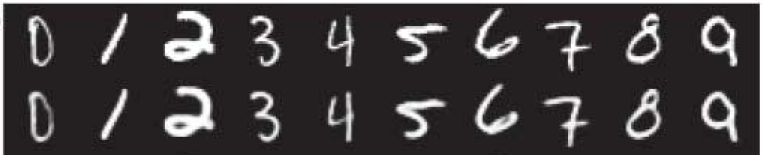
%%%% DISPLAY FIGURE TOP ROW REAL DATA BOTTOM ROW RECONSTRUCTIONS 显示真实的和重构后的数据 %%%%%%%%%%%%%%%%%%%%%%%%%
fprintf(1,'Displaying in figure 1: Top row - real data, Bottom row -- reconstructions
'); %上面一行是真实数据,下面一行是重构数据
output=[];
for ii=1:15 %每次显示15组图片
output = [output data(ii,1:end-1)' dataout(ii,:)']; %两列真实数据和重构后的数据%output为15(因为是显示15个数字)组,每组2列,分别为理论值和重构值
end
if epoch==1
close all
figure('Position',[100,600,1000,200]);
else
figure(1)
end
mnistdisp(output); %画图 展示一组图
drawnow;
%%%%%%%%%%%%%%%%%%%% COMPUTE TEST RECONSTRUCTION ERROR 计算测试重构误差%%%%%%%%%%%%%%%%%%%%%%%%%%%%%%%%%%%%
[testnumcases testnumdims testnumbatches]=size(testbatchdata);%批数% [100 784 100] 测试数据为100个batch,每个batch含100个测试样本,每个样本维数为784
N=testnumcases;
err=0;
for batch = 1:testnumbatches
data = [testbatchdata(:,:,batch)];
data = [data ones(N,1)];
w1probs = 1./(1 + exp(-data*w1)); w1probs = [w1probs ones(N,1)];
w2probs = 1./(1 + exp(-w1probs*w2)); w2probs = [w2probs ones(N,1)];
w3probs = 1./(1 + exp(-w2probs*w3)); w3probs = [w3probs ones(N,1)];
w4probs = w3probs*w4; w4probs = [w4probs ones(N,1)]; %没有把4个RBM展开前输出层神经元(即:第4个rbm的隐含层神经元)的激活函数是f(x)=x,而不是原来的logistic函数。所以把4个RBM展开并连接起来变为9层神经网络后,它的第5层神经元的激活函数仍然是f(x)=x。
w5probs = 1./(1 + exp(-w4probs*w5)); w5probs = [w5probs ones(N,1)];
w6probs = 1./(1 + exp(-w5probs*w6)); w6probs = [w6probs ones(N,1)];
w7probs = 1./(1 + exp(-w6probs*w7)); w7probs = [w7probs ones(N,1)];
dataout = 1./(1 + exp(-w7probs*w8)); %输出层的输出概率密度=重构数据的概率密度=重构数据
err = err + 1/N*sum(sum( (data(:,1:end-1)-dataout).^2 ));
end
test_err(epoch)=err/testnumbatches;
fprintf(1,'Before epoch %d Train squared error: %6.3f Test squared error: %6.3f
',epoch,train_err(epoch),test_err(epoch));
%%%%%%%%%%%%%% END OF COMPUTING TEST RECONSTRUCTION ERROR 测试重构误差计算结束%%%%%%%%%%%%%%%%%%%%%%%%%%%%%%%%%%
%%组合数据的batches大小由原来的100*600的mini-batches变为1000*60的larger-batches
tt=0;
for batch = 1:numbatches/10% 训练样本:批数numbatches是600,每个batch内100个样本,组合后变为批数60,每个batch1000个样本
fprintf(1,'epoch %d batch %d
',epoch,batch);
%%%%%%%%%%% COMBINE 10 MINIBATCHES INTO 1 LARGER MINIBATCH 将10个小批合并为1个较大的小批%%%%%%%%%%%%%%%%%%%%%%%%%%%%%%%%%
tt=tt+1;
data=[];
for kk=1:10
data=[data
batchdata(:,:,(tt-1)*10+kk)]; %将10个100行数据连成一行%使训练数据变为60个batch,每个batch内含1000个样本
end
%%%%%%%%%%%%%%% PERFORM CONJUGATE GRADIENT WITH 3 LINESEARCHES 共轭梯度%%%%%%%%%%%%%%%%%%%%%%%%%%%%%
max_iter=3; %3次线性搜索
% VV将权值偏置矩阵展成一个长长的列向量
VV = [w1(:)' w2(:)' w3(:)' w4(:)' w5(:)' w6(:)' w7(:)' w8(:)']'; %将所有的权值和偏置合并为1列% 把所有权值(已经包括了偏置值)变成一个大的列向量
Dim = [l1; l2; l3; l4; l5; l6; l7; l8; l9]; %所有结点 每层节点个数% 每层网络对应节点的个数(不包括偏置值)
[X, fX] = minimize(VV,'CG_MNIST',max_iter,Dim,data);%实现共轭梯度% X为3次线性搜索最优化后得到的权值参数,是一个列向量
%VV是权值偏置 CG_MNIST输出的是代价函数和偏导 结点 数据
% 将VV列向量重新还原成矩阵
w1 = reshape(X(1:(l1+1)*l2),l1+1,l2); %(l1+1)*l2 (784+1)*1000
xxx = (l1+1)*l2;
w2 = reshape(X(xxx+1:xxx+(l2+1)*l3),l2+1,l3);
xxx = xxx+(l2+1)*l3;
w3 = reshape(X(xxx+1:xxx+(l3+1)*l4),l3+1,l4);
xxx = xxx+(l3+1)*l4;
w4 = reshape(X(xxx+1:xxx+(l4+1)*l5),l4+1,l5);
xxx = xxx+(l4+1)*l5;
w5 = reshape(X(xxx+1:xxx+(l5+1)*l6),l5+1,l6);
xxx = xxx+(l5+1)*l6;
w6 = reshape(X(xxx+1:xxx+(l6+1)*l7),l6+1,l7);
xxx = xxx+(l6+1)*l7;
w7 = reshape(X(xxx+1:xxx+(l7+1)*l8),l7+1,l8);
xxx = xxx+(l7+1)*l8;
w8 = reshape(X(xxx+1:xxx+(l8+1)*l9),l8+1,l9);%依次重新赋值为优化后的参数
%%%%%%%%%%%%%%% END OF CONJUGATE GRADIENT WITH 3 LINESEARCHES %%%%%%%%%%%%%%%%%%%%%%%%%%%%%
end
save mnist_weights w1 w2 w3 w4 w5 w6 w7 w8
save mnist_error test_err train_err;
end
6.CG_MNIST.m
%该函数实现的功能是计算网络代价函数值f,以及f对网络中各个参数值的偏导数df,权值和偏置值是同时处理。
%其中参数VV为网络中所有参数构成的列向量,参数Dim为每层网络的节点数构成的向量,XX为训练样本集合。f和df分别表示网络的代价函数和偏导函数值。
%得代价函数和对权值的偏导数
function [f, df] = CG_MNIST(VV,Dim,XX) %权值,结点,输入数据
% f :代价函数,即交叉熵误差 -1/N*∑∑(X*log(H)+(1-X)*log(1-H))
% df :代价函数对各权值的偏导数
% VV:权值(已经包括了偏置值),为一个大的列向量 用预训练初始的权值与偏置
% Dim:每层网络对应节点的个数
% XX:训练样本
% f :代价函数,即交叉熵误差
% df :代价函数对各权值的偏导数
l1 = Dim(1);%各层节点个数(不包括偏置值) 784
l2 = Dim(2);  %1000
l3 = Dim(3);  %500
l4= Dim(4);  %250
l5= Dim(5);  %30
l6= Dim(6);  %250
l7= Dim(7);  %500
l8= Dim(8);  %1000
l9= Dim(9);  %784
N = size(XX,1);% 样本的个数
% Do decomversion. 权值矩阵化
 w1 = reshape(VV(1:(l1+1)*l2),l1+1,l2); %依次取出每层的权值和偏置% VV是一个长的列向量,它包括偏置值和权值,这里取出的向量已经包括了偏置值 785*1000
 xxx = (l1+1)*l2;%xxx 表示已经使用了的长度
 w2 = reshape(VV(xxx+1:xxx+(l2+1)*l3),l2+1,l3); %1001*500
 xxx = xxx+(l2+1)*l3;
 w3 = reshape(VV(xxx+1:xxx+(l3+1)*l4),l3+1,l4);  %501*250
 xxx = xxx+(l3+1)*l4;
 w4 = reshape(VV(xxx+1:xxx+(l4+1)*l5),l4+1,l5);  %251*30
 xxx = xxx+(l4+1)*l5;
 w5 = reshape(VV(xxx+1:xxx+(l5+1)*l6),l5+1,l6);  %31*250
 xxx = xxx+(l5+1)*l6;
 w6 = reshape(VV(xxx+1:xxx+(l6+1)*l7),l6+1,l7);  %251*500
 xxx = xxx+(l6+1)*l7;
 w7 = reshape(VV(xxx+1:xxx+(l7+1)*l8),l7+1,l8);  %501*1000
 xxx = xxx+(l7+1)*l8;
 w8 = reshape(VV(xxx+1:xxx+(l8+1)*l9),l8+1,l9);  %1001*784
  XX = [XX ones(N,1)];% 训练样本,加1维使其下可乘w1
  w1probs = 1./(1 + exp(-XX*w1)); w1probs = [w1probs  ones(N,1)];
  w2probs = 1./(1 + exp(-w1probs*w2)); w2probs = [w2probs ones(N,1)];
  w3probs = 1./(1 + exp(-w2probs*w3)); w3probs = [w3probs  ones(N,1)];
  w4probs = w3probs*w4; w4probs = [w4probs  ones(N,1)];% 第5层神经元激活函数为1,而不是logistic函数
  w5probs = 1./(1 + exp(-w4probs*w5)); w5probs = [w5probs  ones(N,1)];
  w6probs = 1./(1 + exp(-w5probs*w6)); w6probs = [w6probs  ones(N,1)];
  w7probs = 1./(1 + exp(-w6probs*w7)); w7probs = [w7probs  ones(N,1)];
  XXout = 1./(1 + exp(-w7probs*w8));  %输出的概率密度% 输出层的概率密度,也就是重构数据
%看邱锡鹏: 神经网络与深度学习 P100
%计算每一层参数的导数
f = -1/N*sum(sum( XX(:,1:end-1).*log(XXout) + (1-XX(:,1:end-1)).*log(1-XXout)));  %代价函数交叉熵 -1/N*∑∑(X*log(H)+(1-X)*log(1-H))
IO = 1/N*(XXout-XX(:,1:end-1));  %误差项
Ix8=IO;% 相当于输出层“残差”
dw8 =  w7probs'*Ix8;  %向后推导输出层偏导  W8的偏导=激活值(f(aW+b))'*残差项
Ix7 = (Ix8*w8').*w7probs.*(1-w7probs); %第七层残差
Ix7 = Ix7(:,1:end-1); %误差项
dw7 =  w6probs'*Ix7;  %第七层偏导=激活值(f(aW+b))'*残差项
Ix6 = (Ix7*w7').*w6probs.*(1-w6probs);
Ix6 = Ix6(:,1:end-1); %误差项
dw6 =  w5probs'*Ix6;
Ix5 = (Ix6*w6').*w5probs.*(1-w5probs);
Ix5 = Ix5(:,1:end-1);
dw5 =  w4probs'*Ix5;
Ix4 = (Ix5*w5');
Ix4 = Ix4(:,1:end-1);
dw4 =  w3probs'*Ix4;
Ix3 = (Ix4*w4').*w3probs.*(1-w3probs);
Ix3 = Ix3(:,1:end-1);
dw3 =  w2probs'*Ix3;
Ix2 = (Ix3*w3').*w2probs.*(1-w2probs);
Ix2 = Ix2(:,1:end-1);
dw2 =  w1probs'*Ix2;
Ix1 = (Ix2*w2').*w1probs.*(1-w1probs);
Ix1 = Ix1(:,1:end-1);
dw1 =  XX'*Ix1;
df = [dw1(:)' dw2(:)' dw3(:)' dw4(:)' dw5(:)' dw6(:)'  dw7(:)'  dw8(:)'  ]'; %网络代价函数的偏导数
7.rbm.m 和minimize.m
rbm.m程序在受限玻尔兹曼机(Restricted Boltzmann Machine)中详细阐述了,minimize.m程序在minimize.m:共轭梯度法更新BP算法权值中详细阐述了。
8. 实验结果
9. 参考文献
[1]Hinton G E, Salakhutdinov R R. Reducing the dimensionality of data with neural networks[J]. science, 2006, 313(5786): 504-507.
[2] Hinton,Training a deep autoencoder or a classifieron MNIST digits.
[3] Hinton,Supporting Online Material.
[4]邱锡鹏,神经网络与深度学习[M]. 2019.