matplotlib教程学习笔记
如何使用tight_layout?
tight_layout作用于ticklabels, axis, labels, titles等Artist
简单的例子
import matplotlib.pyplot as plt
import numpy as np
下面的例子和constrained_layout中的是一样的,notebook没有显示出其中的问题,就是labels被遮挡了
plt.rcParams['savefig.facecolor'] = "0.8"
def example_plot(ax, fontsize=12):
ax.plot([1, 2])
ax.locator_params(nbins=3)
ax.set_xlabel('x-label', fontsize=fontsize)
ax.set_ylabel('y-label', fontsize=fontsize)
ax.set_title('Title', fontsize=fontsize)
plt.close('all')
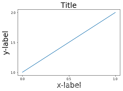
fig, ax = plt.subplots()
example_plot(ax, fontsize=24)
fig, ax = plt.subplots()
example_plot(ax, fontsize=24)
plt.tight_layout()
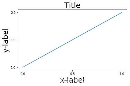
注意到,每次作图,我们都需要通过使用plt.tight_layout()函数来激活,我们也可以通过
fig.set_tight_layout(True)使得每次作图都会自动tight布局,当然,还可以通过将
figure.autolayout rcParam设置为True来实现。
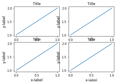
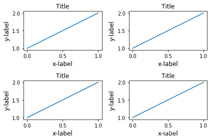
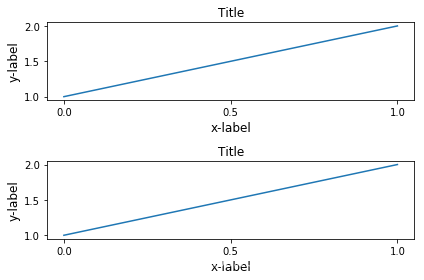
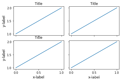
有多个plots的时候,会出现重叠的现象,通过tight_layout可以解决
plt.close('all')

fig, ((ax1, ax2), (ax3, ax4)) = plt.subplots(nrows=2, ncols=2)
example_plot(ax1)
example_plot(ax2)
example_plot(ax3)
example_plot(ax4)
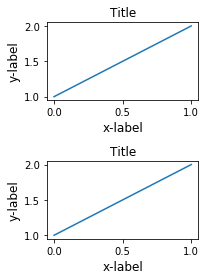
fig, ((ax1, ax2), (ax3, ax4)) = plt.subplots(nrows=2, ncols=2)
example_plot(ax1)
example_plot(ax2)
example_plot(ax3)
example_plot(ax4)
plt.tight_layout()
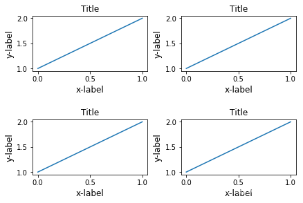
tight_layout可以通过参数pad, w_pad, h_pad来设置一些布局的细节
fig, ((ax1, ax2), (ax3, ax4)) = plt.subplots(nrows=2, ncols=2)
example_plot(ax1)
example_plot(ax2)
example_plot(ax3)
example_plot(ax4)
plt.tight_layout(pad=0.4, w_pad=0.5, h_pad=2)
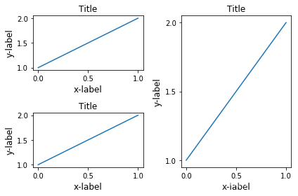
即使subplots的大小不一致,tight_layout依旧能够工作
plt.close('all')
fig = plt.figure()

ax1 = plt.subplot(221)
ax2 = plt.subplot(223)
ax3 = plt.subplot(122)

example_plot(ax1)
example_plot(ax2)
example_plot(ax3)

plt.tight_layout()
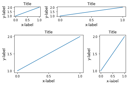
对subplot2grid也有效,注意subplot2grid参数为:
shape: e.g. (3, 3) 表示(3 imes 3)个格子
loc: e.g. (0, 1) 表示从第一行第二列个格子开始
rowspan: 跨行
colspan: 跨列
plt.close('all')
fig = plt.figure()

ax1 = plt.subplot2grid((3, 3), (0, 0))
ax2 = plt.subplot2grid((3, 3), (0, 1), colspan=2)
ax3 = plt.subplot2grid((3, 3), (1, 0), colspan=2, rowspan=2)
ax4 = plt.subplot2grid((3, 3), (1, 2), rowspan=2)

example_plot(ax1)
example_plot(ax2)
example_plot(ax3)
example_plot(ax4)

plt.tight_layout()
arr = np.arange(100).reshape((10, 10))

plt.close('all')
fig = plt.figure(figsize=(5, 4))

ax = plt.subplot(111)
im = ax.imshow(arr, interpolation="none")

plt.tight_layout()
Use with GridSpec
Gridspec 拥有自己的tight_layout()方法, 当然,plt.tight_layout也是有效的
import matplotlib.gridspec as gridspec

plt.close('all')
fig = plt.figure()

gs1 = gridspec.GridSpec(2, 1)
ax1 = fig.add_subplot(gs1[0])
ax2 = fig.add_subplot(gs1[1])

example_plot(ax1)
example_plot(ax2)

gs1.tight_layout(fig)
gs.tight_layout提供rect参数,表示一个外界的框框
默认是(0, 0, 1, 1)
(x1, y1, x2, y2)
(x1, y1)矩形限制框左下角点
(x2, y2)矩形限制框右上角点
fig = plt.figure()

gs1 = gridspec.GridSpec(2, 1)
ax1 = fig.add_subplot(gs1[0])
ax2 = fig.add_subplot(gs1[1])

example_plot(ax1)
example_plot(ax2)

gs1.tight_layout(fig, rect=[0, 0, 0.5, 1])
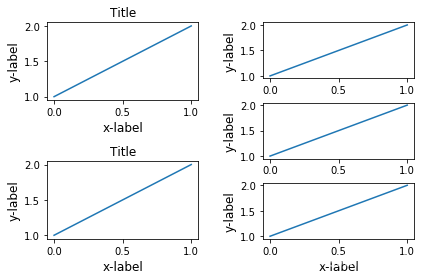
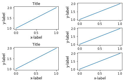
这个功能可以很好的用在分割图形,以及分块操作上
fig = plt.figure()

gs1 = gridspec.GridSpec(2, 1)
ax1 = fig.add_subplot(gs1[0])
ax2 = fig.add_subplot(gs1[1])

example_plot(ax1)
example_plot(ax2)

gs1.tight_layout(fig, rect=[0, 0, 0.5, 1])

gs2 = gridspec.GridSpec(3, 1)

for ss in gs2:
    ax = fig.add_subplot(ss)
    example_plot(ax)
    ax.set_title("")
    ax.set_xlabel("")

ax.set_xlabel("x-label", fontsize=12)

gs2.tight_layout(fig, rect=[0.5, 0, 1, 1], h_pad=0.5)

# We may try to match the top and bottom of two grids ::
#为了让俩块图形上下一致,需要进行下面的操作
top = min(gs1.top, gs2.top)
bottom = max(gs1.bottom, gs2.bottom)

gs1.update(top=top, bottom=bottom)
gs2.update(top=top, bottom=bottom)
plt.show()
但是呢,Title和右边的边边不齐,所以框框是不包含title的?
fig = plt.gcf()

gs1 = gridspec.GridSpec(2, 1)
ax1 = fig.add_subplot(gs1[0])
ax2 = fig.add_subplot(gs1[1])

example_plot(ax1)
example_plot(ax2)

gs1.tight_layout(fig, rect=[0, 0, 0.5, 1])

gs2 = gridspec.GridSpec(3, 1)

for ss in gs2:
    ax = fig.add_subplot(ss)
    example_plot(ax)
    ax.set_title("")
    ax.set_xlabel("")

ax.set_xlabel("x-label", fontsize=12)

gs2.tight_layout(fig, rect=[0.5, 0, 1, 1], h_pad=0.5)

top = min(gs1.top, gs2.top)
bottom = max(gs1.bottom, gs2.bottom)

gs1.update(top=top, bottom=bottom)
gs2.update(top=top, bottom=bottom)

top = min(gs1.top, gs2.top)
bottom = max(gs1.bottom, gs2.bottom)

gs1.tight_layout(fig, rect=[None, 0 + (bottom-gs1.bottom),
                            0.5, 1 - (gs1.top-top)])
gs2.tight_layout(fig, rect=[0.5, 0 + (bottom-gs2.bottom),
                            None, 1 - (gs2.top-top)],
                 h_pad=0.5)
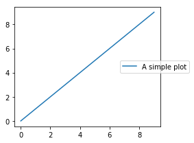
Legend and Annotations
fig, ax = plt.subplots(figsize=(4, 3))
lines = ax.plot(range(10), label='A simple plot')
ax.legend(bbox_to_anchor=(0.7, 0.5), loc='center left',)
fig.tight_layout()
plt.show()
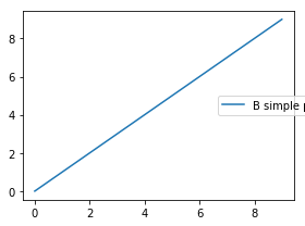
有些时候,我们不希望legend也在tight_layout的掌控范围之内,这个时候,我们可以设置leg.set_in_layout(False)
fig, ax = plt.subplots(figsize=(4, 3))
lines = ax.plot(range(10), label='B simple plot')
leg = ax.legend(bbox_to_anchor=(0.7, 0.5), loc='center left',)
leg.set_in_layout(False)
fig.tight_layout()
plt.show()
Use with AxesGrid1
没看懂
from mpl_toolkits.axes_grid1 import Grid

plt.close('all')
fig = plt.figure()
grid = Grid(fig, rect=111, nrows_ncols=(2, 2),
            axes_pad=0.25, label_mode='L',
            )

for ax in grid:
    example_plot(ax)
ax.title.set_visible(False)

plt.tight_layout()
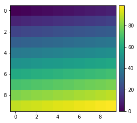
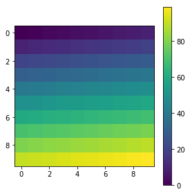
Colorbar
plt.close('all')
arr = np.arange(100).reshape((10, 10))
fig = plt.figure(figsize=(4, 4))
im = plt.imshow(arr, interpolation="none")

plt.colorbar(im, use_gridspec=True)

plt.close('all')
arr = np.arange(100).reshape((10, 10))
fig = plt.figure(figsize=(4, 4))
im = plt.imshow(arr, interpolation="none")

plt.colorbar(im, use_gridspec=True)

plt.tight_layout()
from mpl_toolkits.axes_grid1 import make_axes_locatable

plt.close('all')
arr = np.arange(100).reshape((10, 10))
fig = plt.figure(figsize=(4, 4))
im = plt.imshow(arr, interpolation="none")

divider = make_axes_locatable(plt.gca())
cax = divider.append_axes("right", "5%", pad="3%")
plt.colorbar(im, cax=cax)

plt.tight_layout()