https://www.jianshu.com/p/2e7ffe06fcdd?tdsourcetag=s_pcqq_aiomsg
https://github.com/echen/restricted-boltzmann-machines/blob/master/rbm.py
https://github.com/echen/restricted-boltzmann-machines
http://blog.echen.me/2011/07/18/introduction-to-restricted-boltzmann-machines/
Suppose you ask a bunch of users to rate a set of movies on a 0-100 scale. In classical factor analysis, you could then try to explain each movie and user in terms of a set of latent factors. For example, movies like Star Wars and Lord of the Rings might have strong associations with a latent science fiction and fantasy factor, and users who like Wall-E and Toy Story might have strong associations with a latent Pixar factor.
Restricted Boltzmann Machines essentially perform a binary version of factor analysis. (This is one way of thinking about RBMs; there are, of course, others, and lots of different ways to use RBMs, but I’ll adopt this approach for this post.) Instead of users rating a set of movies on a continuous scale, they simply tell you whether they like a movie or not, and the RBM will try to discover latent factors that can explain the activation of these movie choices.
More technically, a Restricted Boltzmann Machine is a stochastic neural network (neural network meaning we have neuron-like units whose binary activations depend on the neighbors they’re connected to; stochastic meaning these activations have a probabilistic element) consisting of:
- One layer of visible units (users’ movie preferences whose states we know and set);
- One layer of hidden units (the latent factors we try to learn); and
- A bias unit (whose state is always on, and is a way of adjusting for the different inherent popularities of each movie).
Furthermore, each visible unit is connected to all the hidden units (this connection is undirected, so each hidden unit is also connected to all the visible units), and the bias unit is connected to all the visible units and all the hidden units. To make learning easier, we restrict the network so that no visible unit is connected to any other visible unit and no hidden unit is connected to any other hidden unit.
For example, suppose we have a set of six movies (Harry Potter, Avatar, LOTR 3, Gladiator, Titanic, and Glitter) and we ask users to tell us which ones they want to watch. If we want to learn two latent units underlying movie preferences – for example, two natural groups in our set of six movies appear to be SF/fantasy (containing Harry Potter, Avatar, and LOTR 3) and Oscar winners (containing LOTR 3, Gladiator, and Titanic), so we might hope that our latent units will correspond to these categories – then our RBM would look like the following:
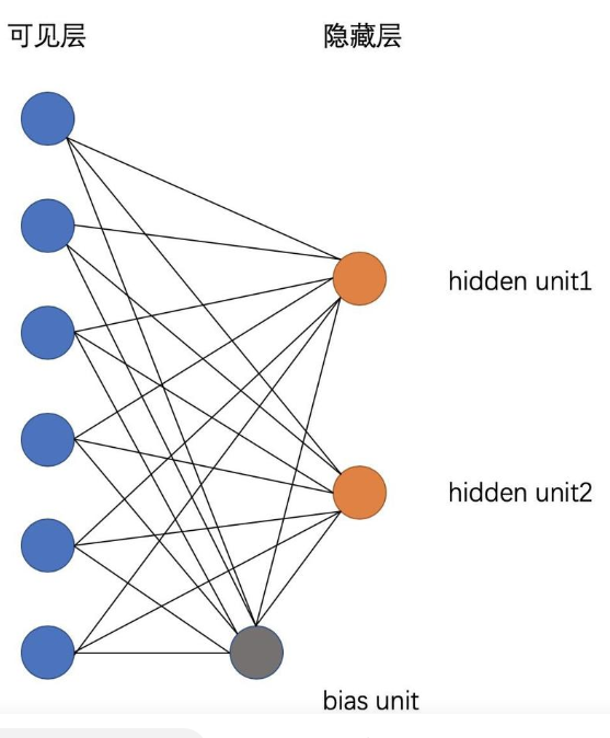
(Note the resemblance to a factor analysis graphical model.)
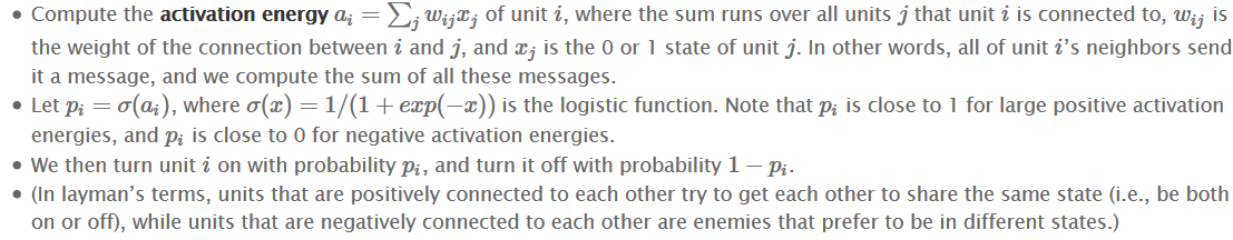
State ActivationRestricted Boltzmann Machines, and neural networks in general, work by updating the states of some neurons given the states of others, so let’s talk about how the states of individual units change. Assuming we know the connection weights in our RBM (we’ll explain how to learn these below), to update the state of unit i
For example, let’s suppose our two hidden units really do correspond to SF/fantasy and Oscar winners.
- If Alice has told us her six binary preferences on our set of movies, we could then ask our RBM which of the hidden units her preferences activate (i.e., ask the RBM to explain her preferences in terms of latent factors). So the six movies send messages to the hidden units, telling them to update themselves. (Note that even if Alice has declared she wants to watch Harry Potter, Avatar, and LOTR 3, this doesn’t guarantee that the SF/fantasy hidden unit will turn on, but only that it will turn on with high probability. This makes a bit of sense: in the real world, Alice wanting to watch all three of those movies makes us highly suspect she likes SF/fantasy in general, but there’s a small chance she wants to watch them for other reasons. Thus, the RBM allows us to generate models of people in the messy, real world.)
- Conversely, if we know that one person likes SF/fantasy (so that the SF/fantasy unit is on), we can then ask the RBM which of the movie units that hidden unit turns on (i.e., ask the RBM to generate a set of movie recommendations). So the hidden units send messages to the movie units, telling them to update their states. (Again, note that the SF/fantasy unit being on doesn’t guarantee that we’ll always recommend all three of Harry Potter, Avatar, and LOTR 3 because, hey, not everyone who likes science fiction liked Avatar.)
So how do we learn the connection weights in our network? Suppose we have a bunch of training examples, where each training example is a binary vector with six elements corresponding to a user’s movie preferences. Then for each epoch, do the following:
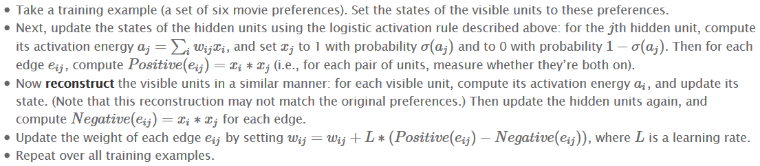
Continue until the network converges (i.e., the error between the training examples and their reconstructions falls below some threshold) or we reach some maximum number of epochs.
Why does this update rule make sense? Note that
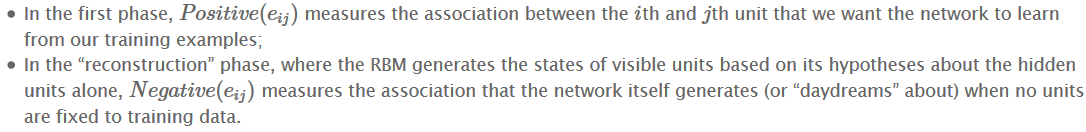
So by adding Positive(eij)−Negative(eij)
to each edge weight, we’re helping the network’s daydreams better match the reality of our training examples.
(You may hear this update rule called contrastive divergence, which is basically a fancy term for “approximate gradient descent”.)
ExamplesI wrote a simple RBM implementation in Python (the code is heavily commented, so take a look if you’re still a little fuzzy on how everything works), so let’s use it to walk through some examples.
First, I trained the RBM using some fake data.
- Alice: (Harry Potter = 1, Avatar = 1, LOTR 3 = 1, Gladiator = 0, Titanic = 0, Glitter = 0). Big SF/fantasy fan.
- Bob: (Harry Potter = 1, Avatar = 0, LOTR 3 = 1, Gladiator = 0, Titanic = 0, Glitter = 0). SF/fantasy fan, but doesn’t like Avatar.
- Carol: (Harry Potter = 1, Avatar = 1, LOTR 3 = 1, Gladiator = 0, Titanic = 0, Glitter = 0). Big SF/fantasy fan.
- David: (Harry Potter = 0, Avatar = 0, LOTR 3 = 1, Gladiator = 1, Titanic = 1, Glitter = 0). Big Oscar winners fan.
- Eric: (Harry Potter = 0, Avatar = 0, LOTR 3 = 1, Gladiator = 1, Titanic = 1, Glitter = 0). Oscar winners fan, except for Titanic.
- Fred: (Harry Potter = 0, Avatar = 0, LOTR 3 = 1, Gladiator = 1, Titanic = 1, Glitter = 0). Big Oscar winners fan.
The network learned the following weights:

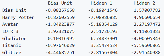
Note that the first hidden unit seems to correspond to the Oscar winners, and the second hidden unit seems to correspond to the SF/fantasy movies, just as we were hoping.
What happens if we give the RBM a new user, George, who has (Harry Potter = 0, Avatar = 0, LOTR 3 = 0, Gladiator = 1, Titanic = 1, Glitter = 0) as his preferences? It turns the Oscar winners unit on (but not the SF/fantasy unit), correctly guessing that George probably likes movies that are Oscar winners.
What happens if we activate only the SF/fantasy unit, and run the RBM a bunch of different times? In my trials, it turned on Harry Potter, Avatar, and LOTR 3 three times; it turned on Avatar and LOTR 3, but not Harry Potter, once; and it turned on Harry Potter and LOTR 3, but not Avatar, twice. Note that, based on our training examples, these generated preferences do indeed match what we might expect real SF/fantasy fans want to watch.
ModificationsI tried to keep the connection-learning algorithm I described above pretty simple, so here are some modifications that often appear in practice:

### from https://github.com/echen/restricted-boltzmann-machines/blob/master/rbm.py
from __future__ import print_function
import numpy as np


class RBM:

    def __init__(self, num_visible, num_hidden):
        self.num_hidden = num_hidden
        self.num_visible = num_visible
        self.debug_print = True

        # Initialize a weight matrix, of dimensions (num_visible x num_hidden), using
        # a uniform distribution between -sqrt(6. / (num_hidden + num_visible))
        # and sqrt(6. / (num_hidden + num_visible)). One could vary the
        # standard deviation by multiplying the interval with appropriate value.
        # Here we initialize the weights with mean 0 and standard deviation 0.1.
        # Reference: Understanding the difficulty of training deep feedforward
        # neural networks by Xavier Glorot and Yoshua Bengio
        np_rng = np.random.RandomState(1234)

        self.weights = np.asarray(np_rng.uniform(
            low=-0.1 * np.sqrt(6. / (num_hidden + num_visible)),
            high=0.1 * np.sqrt(6. / (num_hidden + num_visible)),
            size=(num_visible, num_hidden)))

        # Insert weights for the bias units into the first row and first column.
        self.weights = np.insert(self.weights, 0, 0, axis=0)
        self.weights = np.insert(self.weights, 0, 0, axis=1)

    def train(self, data, max_epochs=1000, learning_rate=0.1):
        """
        Train the machine.
        Parameters
        ----------
        data: A matrix where each row is a training example consisting of the states of visible units.
        """

        num_examples = data.shape[0]

        # Insert bias units of 1 into the first column.
        data = np.insert(data, 0, 1, axis=1)

        for epoch in range(max_epochs):
            # Clamp to the data and sample from the hidden units.
            # (This is the "positive CD phase", aka the reality phase.)
            pos_hidden_activations = np.dot(data, self.weights)
            pos_hidden_probs = self._logistic(pos_hidden_activations)
            pos_hidden_probs[:, 0] = 1  # Fix the bias unit.
            pos_hidden_states = pos_hidden_probs > np.random.rand(num_examples, self.num_hidden + 1)
            # Note that we're using the activation *probabilities* of the hidden states, not the hidden states
            # themselves, when computing associations. We could also use the states; see section 3 of Hinton's
            # "A Practical Guide to Training Restricted Boltzmann Machines" for more.
            pos_associations = np.dot(data.T, pos_hidden_probs)

            # Reconstruct the visible units and sample again from the hidden units.
            # (This is the "negative CD phase", aka the daydreaming phase.)
            neg_visible_activations = np.dot(pos_hidden_states, self.weights.T)
            neg_visible_probs = self._logistic(neg_visible_activations)
            neg_visible_probs[:, 0] = 1  # Fix the bias unit.
            neg_hidden_activations = np.dot(neg_visible_probs, self.weights)
            neg_hidden_probs = self._logistic(neg_hidden_activations)
            # Note, again, that we're using the activation *probabilities* when computing associations, not the states
            # themselves.
            neg_associations = np.dot(neg_visible_probs.T, neg_hidden_probs)

            # Update weights.
            self.weights += learning_rate * ((pos_associations - neg_associations) / num_examples)

            error = np.sum((data - neg_visible_probs) ** 2)
            if self.debug_print:
                print("Epoch %s: error is %s" % (epoch, error))

    def run_visible(self, data):
        """
        Assuming the RBM has been trained (so that weights for the network have been learned),
        run the network on a set of visible units, to get a sample of the hidden units.

        Parameters
        ----------
        data: A matrix where each row consists of the states of the visible units.

        Returns
        -------
        hidden_states: A matrix where each row consists of the hidden units activated from the visible
        units in the data matrix passed in.
        """

        num_examples = data.shape[0]

        # Create a matrix, where each row is to be the hidden units (plus a bias unit)
        # sampled from a training example.
        hidden_states = np.ones((num_examples, self.num_hidden + 1))

        # Insert bias units of 1 into the first column of data.
        data = np.insert(data, 0, 1, axis=1)

        # Calculate the activations of the hidden units.
        hidden_activations = np.dot(data, self.weights)
        # Calculate the probabilities of turning the hidden units on.
        hidden_probs = self._logistic(hidden_activations)
        # Turn the hidden units on with their specified probabilities.
        hidden_states[:, :] = hidden_probs > np.random.rand(num_examples, self.num_hidden + 1)
        # Always fix the bias unit to 1.
        # hidden_states[:,0] = 1

        # Ignore the bias units.
        hidden_states = hidden_states[:, 1:]
        return hidden_states

    # TODO: Remove the code duplication between this method and `run_visible`?
    def run_hidden(self, data):
        """
        Assuming the RBM has been trained (so that weights for the network have been learned),
        run the network on a set of hidden units, to get a sample of the visible units.
        Parameters
        ----------
        data: A matrix where each row consists of the states of the hidden units.
        Returns
        -------
        visible_states: A matrix where each row consists of the visible units activated from the hidden
        units in the data matrix passed in.
        """

        num_examples = data.shape[0]

        # Create a matrix, where each row is to be the visible units (plus a bias unit)
        # sampled from a training example.
        visible_states = np.ones((num_examples, self.num_visible + 1))

        # Insert bias units of 1 into the first column of data.
        data = np.insert(data, 0, 1, axis=1)

        # Calculate the activations of the visible units.
        visible_activations = np.dot(data, self.weights.T)
        # Calculate the probabilities of turning the visible units on.
        visible_probs = self._logistic(visible_activations)
        # Turn the visible units on with their specified probabilities.
        visible_states[:, :] = visible_probs > np.random.rand(num_examples, self.num_visible + 1)
        # Always fix the bias unit to 1.
        # visible_states[:,0] = 1

        # Ignore the bias units.
        visible_states = visible_states[:, 1:]
        return visible_states

    def daydream(self, num_samples):
        """
        Randomly initialize the visible units once, and start running alternating Gibbs sampling steps
        (where each step consists of updating all the hidden units, and then updating all of the visible units),
        taking a sample of the visible units at each step.
        Note that we only initialize the network *once*, so these samples are correlated.
        Returns
        -------
        samples: A matrix, where each row is a sample of the visible units produced while the network was
        daydreaming.
        """

        # Create a matrix, where each row is to be a sample of of the visible units
        # (with an extra bias unit), initialized to all ones.
        samples = np.ones((num_samples, self.num_visible + 1))

        # Take the first sample from a uniform distribution.
        samples[0, 1:] = np.random.rand(self.num_visible)

        # Start the alternating Gibbs sampling.
        # Note that we keep the hidden units binary states, but leave the
        # visible units as real probabilities. See section 3 of Hinton's
        # "A Practical Guide to Training Restricted Boltzmann Machines"
        # for more on why.
        for i in range(1, num_samples):
            visible = samples[i - 1, :]

            # Calculate the activations of the hidden units.
            hidden_activations = np.dot(visible, self.weights)
            # Calculate the probabilities of turning the hidden units on.
            hidden_probs = self._logistic(hidden_activations)
            # Turn the hidden units on with their specified probabilities.
            hidden_states = hidden_probs > np.random.rand(self.num_hidden + 1)
            # Always fix the bias unit to 1.
            hidden_states[0] = 1

            # Recalculate the probabilities that the visible units are on.
            visible_activations = np.dot(hidden_states, self.weights.T)
            visible_probs = self._logistic(visible_activations)
            visible_states = visible_probs > np.random.rand(self.num_visible + 1)
            samples[i, :] = visible_states

        # Ignore the bias units (the first column), since they're always set to 1.
        return samples[:, 1:]

    def _logistic(self, x):
        return 1.0 / (1 + np.exp(-x))


if __name__ == '__main__':
    r = RBM(num_visible=6, num_hidden=2)
    training_data = np.array(
        [[1, 1, 1, 0, 0, 0], [1, 0, 1, 0, 0, 0], [1, 1, 1, 0, 0, 0], [0, 0, 1, 1, 1, 0], [0, 0, 1, 1, 0, 0],
         [0, 0, 1, 1, 1, 0]])
    r.train(training_data, max_epochs=5000)
    print(r.weights)
    user = np.array([[0, 0, 0, 1, 1, 0]])
    print(r.run_visible(user))