摘要:
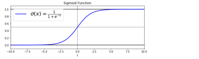
1.基本函数建立1.1 Sigmaid函数:变量和自变量。当我们考虑二值化问题时,因为目标变量只能取0或1,所以我们选择范围在{0,1}区间内的S形函数,也称为Logistic函数,或Logistic Sigmaid函数,也称S曲线1.2问题1.3代码实验importnumpyasnpimportmatplotlib.pyplotaspltimportmatplo
1 基本函数确立
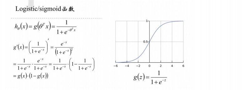
1.1 Sigmoid函数:变量以及自变量
而当我们考虑二值化问题时,由于目标变量只能取0或1,因此我们选择了值域在{0,1}区间的Sigmoid函数
Sigmoid函数又叫做Logistic函数,或者Logistic Sigmoid函数,也被经常称作S型曲线
1.2 提问
1.3 代码实验
import numpy as np
import matplotlib.pyplot as plt
import matplotlib as mpl
t = np.linspace(-10, 10, 100)
sig = 1 / (1 + np.exp(-t))
plt.figure(figsize=(9, 3))
plt.plot([-10, 10], [0, 0], "k-") # 下确线:[-10,10]
plt.plot([-10, 10], [0.5, 0.5], "k:") # 阈值:虚线[0.5,0.5]
plt.plot([-10, 10], [1, 1], "k-")# 上确线:[-10,10]
plt.plot([0, 0], [-1.1, 1.1], "k:") # 中间的分割线
plt.plot(t, sig, "b-", linewidth=2, label=r"$sigma(x) = frac{1}{1 + e^{-x}}$")
plt.xlabel("t")
plt.legend(loc="upper left", fontsize=20)
plt.axis([-10, 10, -0.1, 1.1])
plt.title('Sigmoid Function')
plt.show()

2.确立目标函数
2.1 数学分析工具:最大似然估计/MLE
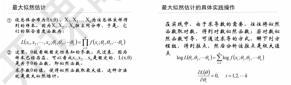
2.2 从统计角度着手


2.3 对数似然函数

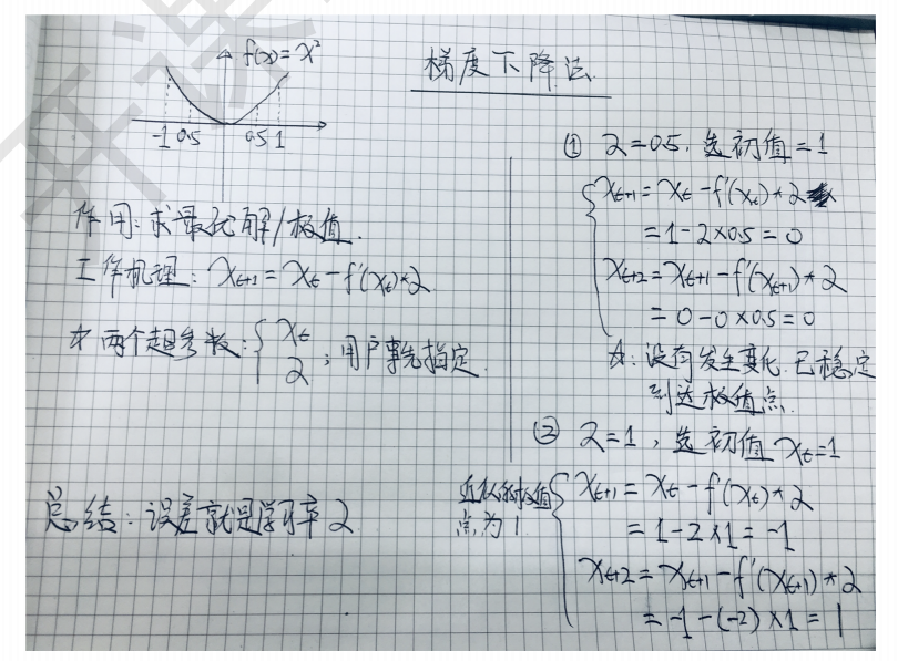
3 确立最优函数
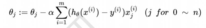
最优方法/工具:梯度下降算法


4.实现逻辑回归算法
4.1 Python着手建模
import pandas as pd
import numpy as np
import matplotlib as mpl
import matplotlib.pyplot as plt

from scipy.optimize import minimize # 求局部最小值
def loaddata(file, delimeter):
    data = np.loadtxt(file, delimiter=delimeter)
    print('显示行列式: ',data.shape)
    print(data[1:6,:]) # 显示5行,所有列
    return(data)
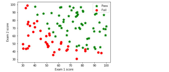
def plotData(data, label_x, label_y, label_pos, label_neg, axes=None):
    # 获得正负样本的下标(即哪些是正样本,哪些是负样本)
    neg = data[:,2] == 0
    pos = data[:,2] == 1

    if axes == None:
        axes = plt.gca() # 得到当前的坐标轴
     #读取所有行的第一列的正样本/1,取所有行的第二列的正样本/1
    axes.scatter(data[pos][:,0], data[pos][:,1], marker='*', c='g', s=60, linewidth=2, label=label_pos)

    #读取所有行的第一列的负样本/0,取所有行的第二列的负样本/0
    axes.scatter(data[neg][:,0], data[neg][:,1], c='r', s=60, label=label_neg)

    axes.set_xlabel(label_x)
    axes.set_ylabel(label_y)
    axes.legend(); # 显示字符或表达式向量
data = loaddata('./data/data1.txt', ',')
显示行列式:  (100, 3)
[[30.28671077 43.89499752  0.        ]
 [35.84740877 72.90219803  0.        ]
 [60.18259939 86.3085521   1.        ]
 [79.03273605 75.34437644  1.        ]
 [45.08327748 56.31637178  0.        ]]
# np.c_是按行连接两个矩阵,就是把两矩阵左右相加,要求行数相等。
# data.shape = (100,3),[0] = 100行 ,加了100行为1

X = np.c_[np.ones((data.shape[0],1)), data[:,0:2]]
y = np.c_[data[:,2]]
plotData(data, 'Exam 1 score', 'Exam 2 score', 'Pass', 'Fail')
#定义sigmoid函数
def sigmoid(z):
    return(1 / (1 + np.exp(-z)))
#定义损失函数
def costFunction(theta, X, y):
    m = y.size

    h = sigmoid(X.dot(theta))

    J = -1.0*(1.0/m)*(np.log(h).T.dot(y)+np.log(1-h).T.dot(1-y))

    if np.isnan(J[0]):
        return(np.inf) # inf:下确界/最小值
    return J[0]
#求偏导
def gradient(theta, X, y):
    m = y.size
    h = sigmoid(X.dot(theta.reshape(-1,1)))

    grad =(1.0/m)*X.T.dot(h-y)

    return(grad.flatten())
import warnings
warnings.filterwarnings("ignore")

initial_theta = np.zeros(X.shape[1])
cost = costFunction(initial_theta, X, y)
grad = gradient(initial_theta, X, y)
print('Cost=', cost)
Cost= 0.6931471805599453
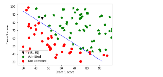
# 预测结果
def predict(theta, X, threshold=0.5):
    p = sigmoid(X.dot(theta.T)) >= threshold
    return(p.astype('int'))
warnings.filterwarnings(action="ignore", category=Warning)
# 最小化损失函数
res = minimize(costFunction, initial_theta, args=(X,y), jac=gradient, options={'maxiter':400})
# 考试1得分45,考试2得分85的同学通过概率有多高
sigmoid(np.array([1,45, 85]).dot(res.x.T))
0.7762903249331021
# 画决策边界
plt.scatter(45, 85, s=60, c='k', marker='v', label='(45, 85)')
plotData(data, 'Exam 1 score', 'Exam 2 score', 'Admitted', 'Not admitted')
x1_min, x1_max = X[:,1].min(), X[:,1].max(),
x2_min, x2_max = X[:,2].min(), X[:,2].max(),
xx1, xx2 = np.meshgrid(np.linspace(x1_min, x1_max), np.linspace(x2_min, x2_max))
h = sigmoid(np.c_[np.ones((xx1.ravel().shape[0],1)), xx1.ravel(), xx2.ravel()].dot(res.x))
h = h.reshape(xx1.shape)
plt.contour(xx1, xx2, h, [0.5], linewidths=1, colors='b');
4.2 Sklearn着手实现
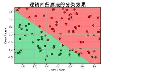
# !/usr/bin/python
# -*- coding:utf-8 -*-

import numpy as np
from sklearn.linear_model import LogisticRegression
import matplotlib.pyplot as plt
import matplotlib as mpl
from sklearn import preprocessing
import pandas as pd
from sklearn.preprocessing import StandardScaler


if __name__ == "__main__":
    path = './data/data1.txt'  # 数据文件路径


    data = np.loadtxt(path, dtype=float, delimiter=',')
#     print(data)

    x, y = np.split(data, (2,), axis=1)
#     print(x)
#     print(y)
# 设置字符集,防止中文乱码
# mpl.rcParams["font.sans-serif"] = [u'simHei'] #Win自带的字体

plt.rcParams['font.sans-serif'] = ['Arial Unicode MS'] #Mac自带的字体
mpl.rcParams["axes.unicode_minus"] = False
    x = StandardScaler().fit_transform(x)
    lr = LogisticRegression().fit(x, y.ravel())   # Logistic回归模型

    # 训练集上的预测结果
    y_hat = lr.predict(x)
    y = y.reshape(-1)
    result = y_hat == y
    print(y_hat)
    print(result)
    acc = np.mean(result)
    print('准确度: %.2f%%' % (100 * acc))
[0. 0. 0. 1. 1. 0. 1. 0. 1. 1. 1. 0. 1. 1. 0. 1. 0. 0. 1. 1. 0. 1. 0. 0.
 1. 1. 1. 1. 0. 0. 1. 1. 0. 0. 0. 0. 1. 1. 0. 0. 1. 0. 1. 1. 0. 0. 1. 1.
 1. 1. 1. 1. 1. 0. 0. 0. 1. 1. 1. 1. 1. 0. 0. 0. 0. 0. 1. 0. 1. 1. 0. 1.
 1. 1. 1. 1. 1. 1. 0. 1. 1. 1. 1. 0. 1. 1. 0. 1. 1. 0. 1. 1. 0. 1. 1. 1.
 1. 1. 0. 1.]
[ True  True  True  True  True  True  True False  True  True False  True
  True  True  True  True False  True  True  True  True  True  True  True
  True  True  True False  True  True  True  True  True False  True  True
 False  True  True  True  True  True  True False  True  True  True  True
  True  True  True  True  True  True  True  True  True False  True  True
  True  True  True  True  True  True  True  True  True  True  True  True
  True  True  True  True  True  True  True False  True  True  True False
  True  True  True  True  True  True  True  True  True  True  True  True
  True  True False  True]
准确度: 89.00%
    # 画图
    N, M = 500, 500     # 横纵各采样多少个值
    x1_min, x1_max = x[:, 0].min(), x[:, 0].max()   # 第0列的范围
    x2_min, x2_max = x[:, 1].min(), x[:, 1].max()   # 第1列的范围
    t1 = np.linspace(x1_min, x1_max, N)
    t2 = np.linspace(x2_min, x2_max, M)
    x1, x2 = np.meshgrid(t1, t2)                    # 生成网格采样点
    x_test = np.stack((x1.flat, x2.flat), axis=1)   # 测试点
    cm_light = mpl.colors.ListedColormap(['#77E0A0', '#FF8080'])
    cm_dark = mpl.colors.ListedColormap(['g', 'r'])
    y_hat = lr.predict(x_test)                  # 预测值
    y_hat = y_hat.reshape(x1.shape)                 # 使之与输入的形状相同
    plt.pcolormesh(x1, x2, y_hat, cmap=cm_light)     # 预测值的显示
    plt.scatter(x[:, 0], x[:, 1], c=y, edgecolors='k', s=50, cmap=cm_dark)    # 样本的显示
    plt.xlabel('Exam 1 score')
    plt.ylabel('Exam 2 score')
    plt.title("逻辑回归算法的分类效果",fontsize = 20)
    plt.xlim(x1_min, x1_max)
    plt.ylim(x2_min, x2_max)
    plt.grid()
    plt.savefig('2.png')
    plt.show()