1.原理
小波变换的计算方法:
1)一维信号:
例如:有a=[5,7,6,8]四个数,并使用b[4]数组来保存结果.
则一级Haar小波变换的结果为:
b[0]=(a[0]+a[1])/2, b[2]=(a[0]-a[1])/2
b[1]=(a[2]+a[3])/2, b[3]=(a[2]-a[3])/2
⚠️计算差均值时也有看见a[1]-a[0]的,只要保持一致应该都可以
由此可知,Haar变换采用的原理是:
A)低频采用和均值,即b[0]和b[1],和均值中均值存储了图像的整体信息
B)高频采用差均值,即b[2]和b[3],用于记录图像的细节信息,这样在重构时能够恢复图像的全部信息
因此上面的例子中
b[0] = (5+7)/2 = 6 , b[1] = (6+8)/2 = 6, b[2] = (5-7)/2 = -1, b[3] = (6-8)/2 = -1
如果要继续进行多级的小波变换:
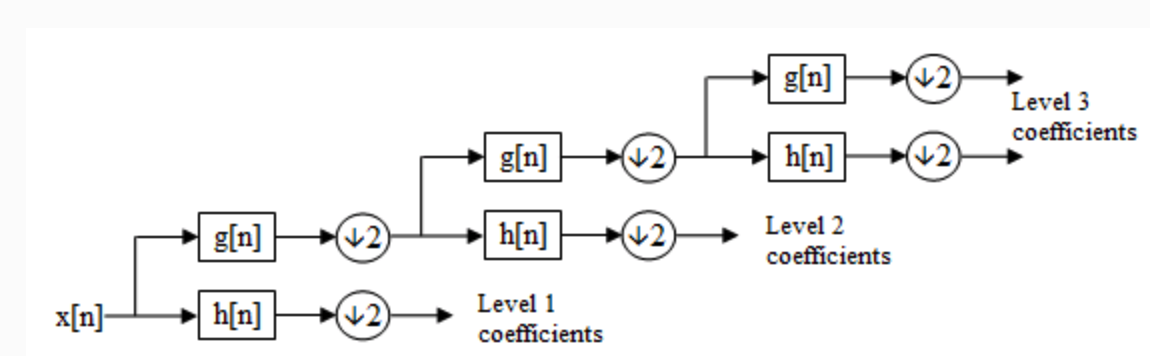
如上图可见是对低频的信息继续进行haar小波变换
2)二维
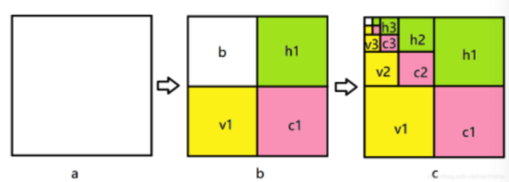
对于二维haar小波,我们通常一次分解形成了整体图像,水平细节,垂直细节,对角细节。首先我们按照一维haar小波分解的原理,按照行顺序对行进行处理,然后按照列顺序对行处理结果进行同样的处理
用图像表述如图所示:图中a表示原图,图b表示经过一级小波变换的结果,h1 表示水平反向的细节,v1 表示竖直方向的细节,c1表示对角线方向的细节,b表示下2采样的图像。图c中表示继续进行了三次Haar小波变换的结果:
详细过程经过下面的代码来解释
2.实现
1)
代码:https://github.com/lpj0/MWCNN_PyTorch/blob/master/model/common.py:
原图为:

中间有个问题,就是逆向重构的时候发现并没有成功,得到的结果是:

于是对操作的数据进行了一番输出:
#coding:utf-8
import torch.nn as nn
import torch

def dwt_init(x):
    print('-------------- origin ---------------')
    print(x[:,0,:,:])
    x01 = x[:, :, 0::2, :] / 2
    x02 = x[:, :, 1::2, :] / 2
    x1 = x01[:, :, :, 0::2]
    x2 = x02[:, :, :, 0::2]
    x3 = x01[:, :, :, 1::2]
    x4 = x02[:, :, :, 1::2]
    x_LL = x1 + x2 + x3 + x4
    x_HL = -x1 - x2 + x3 + x4
    x_LH = -x1 + x2 - x3 + x4
    x_HH = x1 - x2 - x3 + x4
    print('---------------- LL ------------------')
    print(x_LL[:,0,:,:])
    print()
    print('---------------- HL ------------------')
    print(x_HL[:,0,:,:])
    print()
    print('---------------- LH ------------------')
    print(x_LH[:,0,:,:])
    print()
    print('---------------- HH ------------------')
    print(x_HH[:,0,:,:])
    return torch.cat((x_LL, x_HL, x_LH, x_HH), 1)


# 使用哈尔 haar 小波变换来实现二维逆向离散小波
def iwt_init(x):
    r = 2
    in_batch, in_channel, in_height, in_width = x.size()
    # print([in_batch, in_channel, in_height, in_width]) #[1, 12, 56, 56]
    out_batch, out_channel, out_height, out_width = in_batch, int(in_channel / (r**2)), r * in_height, r * in_width
    # print(out_batch, out_channel, out_height, out_width) #1 3 112 112
    x1 = x[:, 0:out_channel, :, :] / 2
    print('-------------- enter iwt ---------------')
    print(x1[:,0,:,:])
    x2 = x[:, out_channel:out_channel * 2, :, :] / 2
    x3 = x[:, out_channel * 2:out_channel * 3, :, :] / 2
    x4 = x[:, out_channel * 3:out_channel * 4, :, :] / 2
    # print(x1.shape) #torch.Size([1, 3, 56, 56])
    # print(x2.shape) #torch.Size([1, 3, 56, 56])
    # print(x3.shape) #torch.Size([1, 3, 56, 56])
    # print(x4.shape) #torch.Size([1, 3, 56, 56])
    # h = torch.zeros([out_batch, out_channel, out_height, out_width]).float().cuda()
    h = torch.zeros([out_batch, out_channel, out_height, out_width]).float()

    h[:, :, 0::2, 0::2] = x1 - x2 - x3 + x4
    h[:, :, 1::2, 0::2] = x1 - x2 + x3 - x4
    h[:, :, 0::2, 1::2] = x1 + x2 - x3 - x4
    h[:, :, 1::2, 1::2] = x1 + x2 + x3 + x4
    print('-------------- back ---------------')
    print(h[:,0,:,:])
    return h


# 二维离散小波
class DWT(nn.Module):
    def __init__(self):
        super(DWT, self).__init__()
        self.requires_grad = False  # 信号处理,非卷积运算,不需要进行梯度求导

    def forward(self, x):
        return dwt_init(x)


# 逆向二维离散小波
class IWT(nn.Module):
    def __init__(self):
        super(IWT, self).__init__()
        self.requires_grad = False

    def forward(self, x):
        return iwt_init(x)

if __name__ == '__main__':
    import os, cv2, torchvision
    from PIL import Image
    import numpy as np
    from torchvision import transforms as trans

    img = Image.open('./1.jpg')
    transform = trans.Compose([
        trans.ToTensor()
    ])
    img = transform(img).unsqueeze(0)
    dwt = DWT()
    change_img_tensor = dwt(img)
    # print(change_img_tensor.shape) #torch.Size([1, 12, 56, 56])
    print('-------------- after dwt ---------------')
    print(change_img_tensor[:,0,:,:])

    for i in range(change_img_tensor.size(1)//3):
        torchvision.utils.save_image(change_img_tensor[:,i*3:i*3+3:,:], os.path.join('./', 'change_{}.jpg'.format(i)))

    iwt = IWT()
    back_img_tensor = iwt(change_img_tensor)
    print(back_img_tensor.shape)

    torchvision.utils.save_image(back_img_tensor, 'back.jpg')
返回:
(deeplearning) bogon:learning user$ python delete.py
-------------- origin ---------------
tensor([[[0.9020, 0.9882, 0.9216,  ..., 0.7176, 0.7843, 0.8431],
         [0.8941, 0.9608, 0.9255,  ..., 0.7490, 0.7569, 0.7490],
         [0.8980, 0.9333, 0.8863,  ..., 0.6941, 0.7333, 0.7608],
         ...,
         [0.1373, 0.1373, 0.1451,  ..., 0.9529, 0.9686, 0.9804],
         [0.1451, 0.1451, 0.1490,  ..., 0.9294, 0.9373, 0.9569],
         [0.1373, 0.1412, 0.1451,  ..., 0.9137, 0.9020, 0.9176]]])
---------------- LL ------------------
tensor([[[1.8725, 1.8569, 1.9314,  ..., 1.4176, 1.4510, 1.5667],
         [1.8294, 1.7588, 1.5118,  ..., 1.4490, 1.4314, 1.5137],
         [1.9039, 1.6059, 1.0412,  ..., 1.2765, 1.4588, 1.5039],
         ...,
         [0.3078, 0.3216, 0.3490,  ..., 1.8784, 1.8333, 1.7627],
         [0.2647, 0.3059, 0.3784,  ..., 1.7510, 1.8725, 1.9137],
         [0.2843, 0.3020, 0.3922,  ..., 1.8941, 1.8549, 1.8569]]])

---------------- HL ------------------
tensor([[[ 0.0765,  0.0098,  0.0059,  ...,  0.0098,  0.0157,  0.0255],
         [ 0.0294, -0.0294, -0.0922,  ..., -0.0098,  0.0078,  0.0235],
         [-0.0412, -0.1588, -0.0725,  ...,  0.0569,  0.0314, -0.0059],
         ...,
         [-0.0137,  0.0196,  0.0039,  ...,  0.0275, -0.0412,  0.0098],
         [-0.0020,  0.0196,  0.0176,  ...,  0.0216,  0.0216,  0.0039],
         [ 0.0020,  0.0078,  0.0314,  ...,  0.0039, -0.0118,  0.0176]]])

---------------- LH ------------------
tensor([[[-0.0176,  0.0098, -0.0176,  ..., -0.0137,  0.0392, -0.0608],
         [-0.0020, -0.0098, -0.1510,  ...,  0.1078,  0.0745,  0.0196],
         [ 0.0176, -0.1392, -0.0882,  ..., -0.0059,  0.0588,  0.0725],
         ...,
         [-0.0255, -0.0078,  0.0118,  ..., -0.0431,  0.0216, -0.0098],
         [ 0.0098,  0.0000,  0.0020,  ...,  0.0020, -0.0020,  0.0353],
         [-0.0059, -0.0039,  0.0039,  ...,  0.0549,  0.0039, -0.0373]]])

---------------- HH ------------------
tensor([[[-0.0098,  0.0059, -0.0216,  ...,  0.0216, -0.0078, -0.0333],
         [-0.0059, -0.0255, -0.0294,  ...,  0.0137, -0.0235, -0.0039],
         [-0.0373, -0.0373,  0.0608,  ..., -0.0020,  0.0196, -0.0098],
         ...,
         [ 0.0059,  0.0039,  0.0039,  ...,  0.0118,  0.0137, -0.0137],
         [ 0.0020, -0.0039,  0.0020,  ..., -0.0098,  0.0137,  0.0078],
         [ 0.0020,  0.0000,  0.0039,  ...,  0.0000, -0.0196, -0.0020]]])
-------------- after dwt ---------------
tensor([[[1.8725, 1.8569, 1.9314,  ..., 1.4176, 1.4510, 1.5667],
         [1.8294, 1.7588, 1.5118,  ..., 1.4490, 1.4314, 1.5137],
         [1.9039, 1.6059, 1.0412,  ..., 1.2765, 1.4588, 1.5039],
         ...,
         [0.3078, 0.3216, 0.3490,  ..., 1.8784, 1.8333, 1.7627],
         [0.2647, 0.3059, 0.3784,  ..., 1.7510, 1.8725, 1.9137],
         [0.2843, 0.3020, 0.3922,  ..., 1.8941, 1.8549, 1.8569]]])
-------------- enter iwt ---------------
tensor([[[127.5000, 127.5000, 127.5000,  ..., 127.5000, 127.5000, 127.5000],
         [127.5000, 127.5000, 127.5000,  ..., 127.5000, 127.5000, 127.5000],
         [127.5000, 127.5000, 127.5000,  ..., 127.5000, 127.5000, 127.5000],
         ...,
         [ 39.5000,  41.2500,  44.7500,  ..., 127.5000, 127.5000, 127.5000],
         [ 34.0000,  39.2500,  48.5000,  ..., 127.5000, 127.5000, 127.5000],
         [ 36.5000,  38.7500,  50.2500,  ..., 127.5000, 127.5000, 127.5000]]])
-------------- back ---------------
tensor([[[117.5000, 137.5000, 125.5000,  ..., 124.5000, 124.0000, 131.0000],
         [117.5000, 137.5000, 126.5000,  ..., 135.0000, 124.0000, 131.0000],
         [123.5000, 131.5000, 127.5000,  ..., 119.0000, 121.5000, 128.0000],
         ...,
         [ 35.0000,  36.0000,  36.7500,  ..., 132.5000, 130.2500, 134.2500],
         [ 36.5000,  36.5000,  37.7500,  ..., 126.7500, 125.0000, 130.0000],
         [ 35.5000,  37.5000,  37.2500,  ..., 128.2500, 125.0000, 130.0000]]])
torch.Size([1, 3, 112, 112])
发现输入iwt的结果变化了,突然想起来torchvision.utils.save_image函数是会对数据进行处理的
解决办法就是调整下顺序即可
重新运行一遍:
#coding:utf-8
import torch.nn as nn
import torch

def dwt_init(x):
    x01 = x[:, :, 0::2, :] / 2
    x02 = x[:, :, 1::2, :] / 2
    x1 = x01[:, :, :, 0::2]
    x2 = x02[:, :, :, 0::2]
    x3 = x01[:, :, :, 1::2]
    x4 = x02[:, :, :, 1::2]
    x_LL = x1 + x2 + x3 + x4
    x_HL = -x1 - x2 + x3 + x4
    x_LH = -x1 + x2 - x3 + x4
    x_HH = x1 - x2 - x3 + x4

    return torch.cat((x_LL, x_HL, x_LH, x_HH), 1)


# 使用哈尔 haar 小波变换来实现二维逆向离散小波
def iwt_init(x):
    r = 2
    in_batch, in_channel, in_height, in_width = x.size()
    # print([in_batch, in_channel, in_height, in_width]) #[1, 12, 56, 56]
    out_batch, out_channel, out_height, out_width = in_batch, int(in_channel / (r**2)), r * in_height, r * in_width
    # print(out_batch, out_channel, out_height, out_width) #1 3 112 112
    x1 = x[:, 0:out_channel, :, :] / 2
    x2 = x[:, out_channel:out_channel * 2, :, :] / 2
    x3 = x[:, out_channel * 2:out_channel * 3, :, :] / 2
    x4 = x[:, out_channel * 3:out_channel * 4, :, :] / 2
    # print(x1.shape) #torch.Size([1, 3, 56, 56])
    # print(x2.shape) #torch.Size([1, 3, 56, 56])
    # print(x3.shape) #torch.Size([1, 3, 56, 56])
    # print(x4.shape) #torch.Size([1, 3, 56, 56])
    # h = torch.zeros([out_batch, out_channel, out_height, out_width]).float().cuda()
    h = torch.zeros([out_batch, out_channel, out_height, out_width]).float()

    h[:, :, 0::2, 0::2] = x1 - x2 - x3 + x4
    h[:, :, 1::2, 0::2] = x1 - x2 + x3 - x4
    h[:, :, 0::2, 1::2] = x1 + x2 - x3 - x4
    h[:, :, 1::2, 1::2] = x1 + x2 + x3 + x4
    return h


# 二维离散小波
class DWT(nn.Module):
    def __init__(self):
        super(DWT, self).__init__()
        self.requires_grad = False  # 信号处理,非卷积运算,不需要进行梯度求导

    def forward(self, x):
        return dwt_init(x)


# 逆向二维离散小波
class IWT(nn.Module):
    def __init__(self):
        super(IWT, self).__init__()
        self.requires_grad = False

    def forward(self, x):
        return iwt_init(x)

if __name__ == '__main__':
    import os, cv2, torchvision
    from PIL import Image
    import numpy as np
    from torchvision import transforms as trans
    # img = cv2.imread('./1.jpg')
    # print(img.shape)
    # img = Image.fromarray(img.astype(np.uint8))
    img = Image.open('./1.jpg')
    transform = trans.Compose([
        trans.ToTensor()
    ])
    img = transform(img).unsqueeze(0)
    dwt = DWT()
    change_img_tensor = dwt(img)
    iwt = IWT()
    back_img_tensor = iwt(change_img_tensor)
    print(back_img_tensor.shape)
    # print(change_img_tensor.shape) #torch.Size([1, 12, 56, 56])


    #合并成一张4格的图
    h = torch.zeros([4,3,change_img_tensor.size(2),change_img_tensor.size(2)]).float()


    for i in range(change_img_tensor.size(1)//3):
        h[i,:,:,:] = change_img_tensor[:,i*3:i*3+3:,:]
        #分别保存为一个图片
        torchvision.utils.save_image(change_img_tensor[:,i*3:i*3+3:,:], os.path.join('./', 'change_{}.jpg'.format(i)))


    change_img_grid = torchvision.utils.make_grid(h, 2) #一行2张图片
    torchvision.utils.save_image(change_img_grid, 'change_img_grid.jpg')

    torchvision.utils.save_image(back_img_tensor, 'back.jpg')
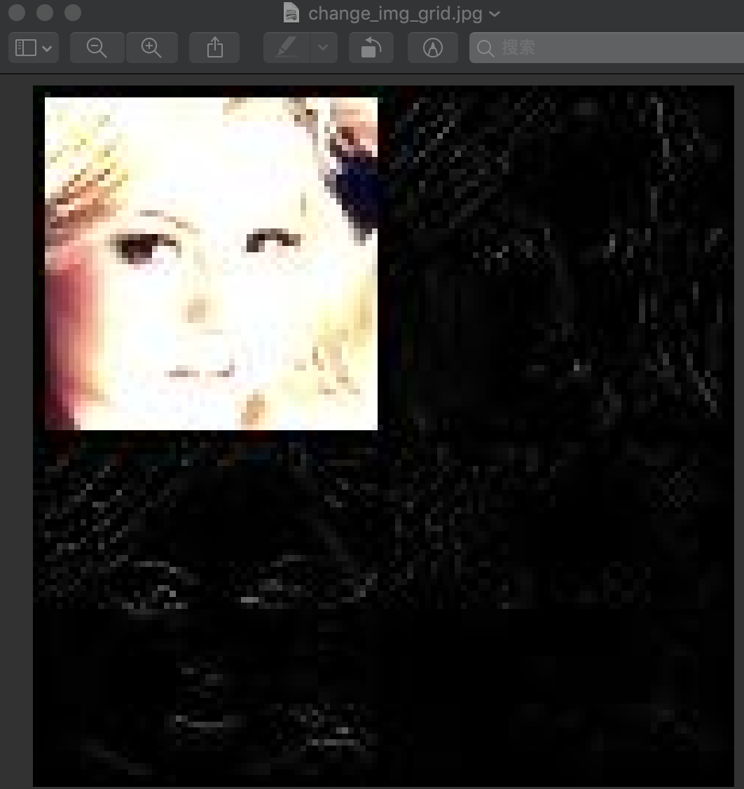
小波变换后的结果为:
重构的图为:

2)对代码进行解释
1》dwt
def dwt_init(x):
    x01 = x[:, :, 0::2, :] / 2
    x02 = x[:, :, 1::2, :] / 2
    x1 = x01[:, :, :, 0::2]
    x2 = x02[:, :, :, 0::2]
    x3 = x01[:, :, :, 1::2]
    x4 = x02[:, :, :, 1::2]
    x_LL = x1 + x2 + x3 + x4
    x_HL = -x1 - x2 + x3 + x4
    x_LH = -x1 + x2 - x3 + x4
    x_HH = x1 - x2 - x3 + x4

    return torch.cat((x_LL, x_HL, x_LH, x_HH), 1)
首先:
    x01 = x[:, :, 0::2, :] / 2
    x02 = x[:, :, 1::2, :] / 2
将矩阵分为偶数行和奇数行,并将所有值都除以2,这样后面只要进行求和和求差即可,因为已经求均值了
然后下面的:
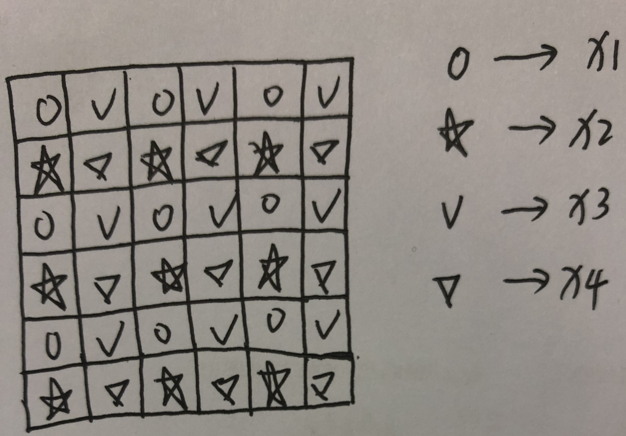
    x1 = x01[:, :, :, 0::2]
    x2 = x02[:, :, :, 0::2]
    x3 = x01[:, :, :, 1::2]
    x4 = x02[:, :, :, 1::2]
就是分为偶数列和奇数列,假设矩阵为6*6大小,那么就将该矩阵分成了4个3*3大小的x1、x2、x3和x4,如下图所示:
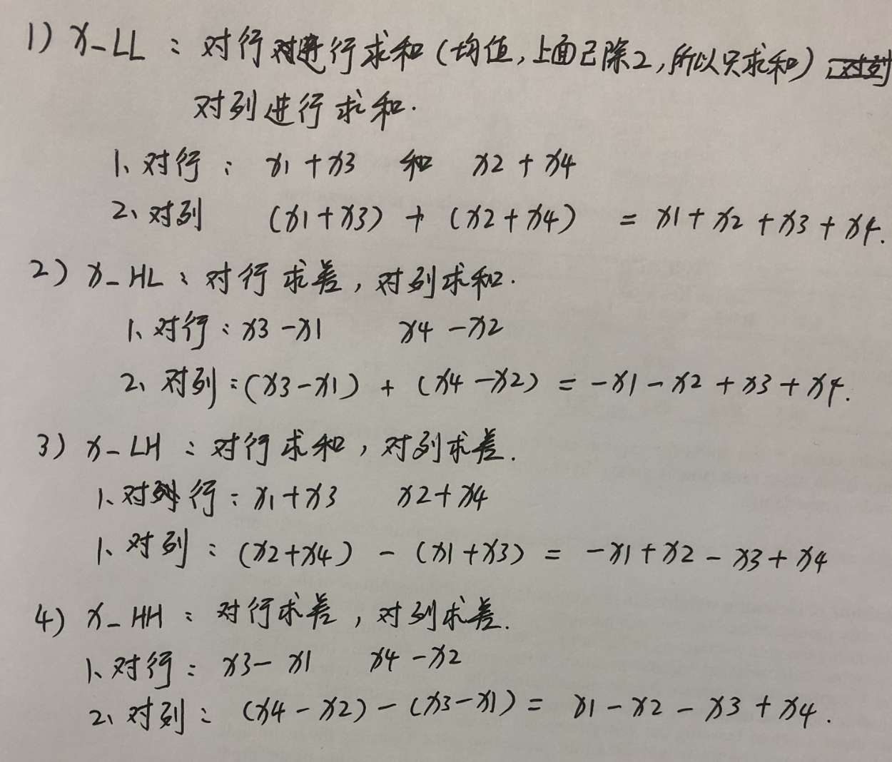
那么接下来在进行的计算就是进行行、列的和、差变换了:
    x_LL = x1 + x2 + x3 + x4
    x_HL = -x1 - x2 + x3 + x4
    x_LH = -x1 + x2 - x3 + x4
    x_HH = x1 - x2 - x3 + x4
再用一张图说明:
2》iwt
def iwt_init(x):
    r = 2
    in_batch, in_channel, in_height, in_width = x.size()
    # print([in_batch, in_channel, in_height, in_width]) #[1, 12, 56, 56]
    out_batch, out_channel, out_height, out_width = in_batch, int(in_channel / (r**2)), r * in_height, r * in_width
    # print(out_batch, out_channel, out_height, out_width) #1 3 112 112
    x1 = x[:, 0:out_channel, :, :] / 2
    x2 = x[:, out_channel:out_channel * 2, :, :] / 2
    x3 = x[:, out_channel * 2:out_channel * 3, :, :] / 2
    x4 = x[:, out_channel * 3:out_channel * 4, :, :] / 2
    # print(x1.shape) #torch.Size([1, 3, 56, 56])
    # print(x2.shape) #torch.Size([1, 3, 56, 56])
    # print(x3.shape) #torch.Size([1, 3, 56, 56])
    # print(x4.shape) #torch.Size([1, 3, 56, 56])
    # h = torch.zeros([out_batch, out_channel, out_height, out_width]).float().cuda()
    h = torch.zeros([out_batch, out_channel, out_height, out_width]).float()

    h[:, :, 0::2, 0::2] = x1 - x2 - x3 + x4
    h[:, :, 1::2, 0::2] = x1 - x2 + x3 - x4
    h[:, :, 0::2, 1::2] = x1 + x2 - x3 - x4
    h[:, :, 1::2, 1::2] = x1 + x2 + x3 + x4
    return h
在这里的行x1=x_LL/2, x2=x_HL/2, x3=x_LH/2, x4=x_HH/2
所以我们想重构,其实就是从这些值中恢复dwt中的x1,x2,x3,x4,分别放到h对应的位置变为原来的矩阵,如x1对应的是h[:, :, 0::2, 0::2],如下图所示:
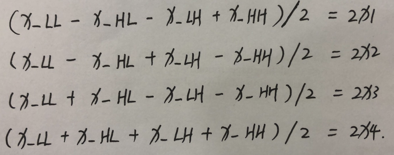
这就是重构的方法
过程中遇到的一点问题pytorch图像处理的问题