作者:zhbzz2007 出处:http://www.cnblogs.com/zhbzz2007 欢迎转载,也请保留这段声明。谢谢!
本文翻译自 RECURRENT NEURAL NETWORKS TUTORIAL, PART 2 – IMPLEMENTING A RNN WITH PYTHON, NUMPY AND THEANO 。
在这篇博文中,我们将会使用Python从头开始实现一个循环神经网络,并且利用Theano(一个在GPU上执行操作的库)优化原始的实现。所有的代码可以在github上获得。我将会跳过一些不影响理解循环神经网络的样例代码,所有这些代码都在github上。
1 语言模型我们的目的就是使用循环神经网络建立语言模型 。假如我们有一个包含m个单词的句子。语言模型允许我们预测在已知数据集中观察到的句子的概率,如下所示,
(P(w_{1},...,w_{m}) = prod_{i=1}^{m}P(w_{i}|w_{1},..w_{i-1}))
总之,一个句子的概率就是每个单词在给定前面的单词后的概率乘积。所以,句子“He went to buy some chocolate”就是给定“He went to buy some”的“chocolate”的概率 乘以 给定“He went to buy”的“some”的概率,等等。
为什么这样就是有用的?为什么我们想要给一个观测到的句子赋予概率?
首先,这类模型可以用作打分机制。例如,一个机器翻译系统对于一个输入句子通常会产生多个候选解。你可以使用语言模型来选择最大可能的句子。直观上,最大可能的句子有可能就是语法正确的。相似的打分在语音识别中也有。
在解决语言模型问题时,也有一个很酷的副产品。因为我们可以预测已知前面词的词的概率,我们也可以生成新的文本。这个就是生成式模型。给定词的序列,我们从预测概率中采样出下一个词,重复这个过程直到我们得到整个句子。Andrej Karparthy的这篇博文很好的显示了语言模型的能力。他的模型是通过单个字符而不是整个单词进行训练的,因此可以生成莎士比亚风格、Linux代码等各种文本。
请注意,上述的公式中每个词的概率是前面所有词的条件概率。实际上,由于计算或者内存限制,许多模型很难表示这么长的依赖。通常的做法是限制到只看前面几个词。理论上,循环神经网络可以获取这么长的依赖,但是在实际中,这个有些复杂,我们将会在后续的博文中介绍。
2 训练数据和预处理为了训练我们的语言模型,我们需要待学习的文本。幸运的是,我们训练语言模型并不需要任何的有标签数据,原始文本就够用了。我从 Google's BigQuery 下载了15,000 条reddit评论数据。通过我们的模型生成的文本,看起来就像reddit的评论。和其它的机器学习项目一样,我们首先对数据进行预处理,将其转换为正确的格式。
2.1 分词
我们手里现在是原始的文本,但是我们想在每个词的基础上进行预测。这就意味着我们需要将评论数据进行分句,然后再对句子进行分词。我们可以通过空格将每条评论进行切分,但是这种方式并不能很好的处理标点符号。句子“He left!”应该是3个词:“He”,“left”,“!”。我们将会使用nltk提供的方法word_tokenize和sent_tokenize来为我们做最为困难的任务,其中word_tokenize用于分词,sent_tokenize用于分句。
2.2 去除低频词
文本中大部分词只出现一次或者两次。将这些低频词删除,是个不错的想法。一个巨大的词汇表将会导致模型的训练速度很慢(我们将会在后面解释原因),并且我们针对这些低频词并没有很多上下文,所以我们无法学习到如何正确的使用它们。这一点很类似于人类学习。为了真正的理解如何合适的使用一个词,你需要在不同的上下文中看到它。
在我们的代码中,我们将词汇表限制为vocabulary_size个常用词(这里我设置为8000,你也可以修改为其它值)。我们将没有出现在词汇表的其它词都替换为 UNKNOWN_TOKEN。例如,如果我们的词汇表没有“nonlinearities”,那么句子“nonlineraties are important in neural networks”就会变为“UNKNOWN_TOKEN are important in neural networks”。词 UNKNOWN_TOKEN将会是词汇表的一部分,我们也会像其他词一样预测它。当我们生成新的文本时,我们可以再次将UNKNOWN_TOKEN替换掉,例如,对词汇表之外的词进行随机采样,或者我们可以只生成句子,直到我们得到一个不包含未知词的句子。
2.3 准备特殊的开始和结束符
我们也想学习哪些词趋向于句子的开始和结束。为了处理这个任务,我们在每个句子的开始加入了 SENTENCE_START 这个词,在句子的结束加入了 SENTENCE_END 这个词。这就会让我们不禁想问:已知第一个词是 SENTENCE_START ,那么下一个最有可能的词(句子中第一个真实的词)是什么?
2.4 建立训练数据矩阵
循环神经网络的输入是向量,而非字符串。所以我们在词和索引之间创建了一个映射,index_to_word 和 word_to_index。例如,词“friendly”的索引或许是2001。一个训练例子 x 或许是[0,179,341,416],0对应 SENTENCE_START 。相应的标签y就是[179,341,416,1]。请记住,我们的目标是预测下一个词,所以 y 就是向量 x 左移一位,最后一个元素是 SENTENCE_END。也就是说,词 179 的正确预测就是 341,也就是真实的下一个词。
代码如下,
vocabulary_size = 8000
unknown_token = "UNKNOWN_TOKEN"
sentence_start_token = "SENTENCE_START"
sentence_end_token = "SENTENCE_END"

# Read the data and append SENTENCE_START and SENTENCE_END tokens
print "Reading CSV file..."
with open('data/reddit-comments-2015-08.csv', 'rb') as f:
    reader = csv.reader(f, skipinitialspace=True)
    reader.next()
    # Split full comments into sentences
    sentences = itertools.chain(*[nltk.sent_tokenize(x[0].decode('utf-8').lower()) for x in reader])
    # Append SENTENCE_START and SENTENCE_END
    sentences = ["%s %s %s" % (sentence_start_token, x, sentence_end_token) for x in sentences]
print "Parsed %d sentences." % (len(sentences))

# Tokenize the sentences into words
tokenized_sentences = [nltk.word_tokenize(sent) for sent in sentences]

# Count the word frequencies
word_freq = nltk.FreqDist(itertools.chain(*tokenized_sentences))
print "Found %d unique words tokens." % len(word_freq.items())

# Get the most common words and build index_to_word and word_to_index vectors
vocab = word_freq.most_common(vocabulary_size-1)
index_to_word = [x[0] for x in vocab]
index_to_word.append(unknown_token)
word_to_index = dict([(w,i) for i,w in enumerate(index_to_word)])

print "Using vocabulary size %d." % vocabulary_size
print "The least frequent word in our vocabulary is '%s' and appeared %d times." % (vocab[-1][0], vocab[-1][1])

# Replace all words not in our vocabulary with the unknown token
for i, sent in enumerate(tokenized_sentences):
    tokenized_sentences[i] = [w if w in word_to_index else unknown_token for w in sent]

print "
Example sentence: '%s'" % sentences[0]
print "
Example sentence after Pre-processing: '%s'" % tokenized_sentences[0]

# Create the training data
X_train = np.asarray([[word_to_index[w] for w in sent[:-1]] for sent in tokenized_sentences])
y_train = np.asarray([[word_to_index[w] for w in sent[1:]] for sent in tokenized_sentences])
下面是文本中真实的训练示例,
x:
SENTENCE_START what are n't you understanding about this ? !
[0, 51, 27, 16, 10, 856, 53, 25, 34, 69]

y:
what are n't you understanding about this ? ! SENTENCE_END
[51, 27, 16, 10, 856, 53, 25, 34, 69, 1]
如果你想对循环神经网络有一个整体的了解,可以阅读 Recurrent Neural Network系列1--RNN(循环神经网络)概述 这篇博文。
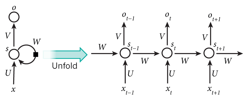
让我们看看用于训练语言模型的循环神经网络具体是什么样子。输入 x 是一个词的序列(就像上面例子的输出) ,每个 (x_{t}) 是一个单独的词。这里还需要注意一件事:由于矩阵相乘,我们不能仅仅使用词的索引作为输入。我们将词表示为一个one-hot向量,向量维度为 vocabulary_size 。例如,表示索引为36的词的向量,所有位置均为0,只有位置36为1。这样,每个 (x_{t}) 将会是一个向量,x将会是一个矩阵,每一行表示一个词。没有在预处理阶段处理,我们将会在神经网络的代码中做这个变换。网络的输出 o 有相似的格式。每个 (o_{t}) 是一个 vocabulary_size 大小的向量,每个元素表示这个词成为句子中下一个词的概率。
我们从第一篇博文中得到循环神经网络的公式,如下所示:
(s_{t} = tanh(U x_{t} + W s_{t-1}))
(o_{t} = softmax(V s_{t}))
我发现将矩阵和向量的维度写出来很有用。假设,我们设置词汇表大小 C = 8000,隐藏层大小 H = 100。你可以将隐藏层大小认为是网络的记忆。让它更大,可以允许我们学习到更加复杂的模式,当然这也会导致额外的计算量。我们将会得到各个矩阵和向量的维度,如下所示,
(x_{t} in R^{8000})
(o_{t} in R^{8000})
(s_{t} in R^{100})
(U in R^{100 * 8000})
(V in R^{8000 * 100})
(W in R^{100 * 100})
这是非常有价值的信息。U,V和W就是我们从数据中学习得到的网络参数。因此,我们总共需要学习 (2*H*C + H^{2}) 个参数。在我们这里,C = 8000,H = 100,总共参数的数量是161万。这个维度也告诉我们模型的瓶颈在哪。由于 (x_{t}) 是一个one-hot向量,将它与 U 进行相乘,就等于选择 U 的某一列,所以我们并不需要执行全部的乘法。网络中最大的矩阵相乘是 (Vs_{t}) 。这也是我们尽可能的让词汇表比较小的原因了。
有了这些,是时候开始我们的实现。
3.1 初始化
我们首先定义RNN类用于初始化我们的参数。我在这里称这个类为RNNNumpy,因为我们将会在后续实现一个基于Theano版本的。初始化U、V、W会有些麻烦。我们不能简单地将它们都初始化为0,因为这样就会导致所有层出现对称的计算。我们必须随机初始化。因为合理的初始化似乎会对训练结果有影响(这个领域已经有很多研究了)。最终发现,最好的初始化依赖于激活函数(我们的例子是tanh),有一个推荐的初始化方法就是在区间 ([-frac{1}{sqrt{n}},frac{1}{sqrt{n}}]) 内初始化权重,这里n是上一层的输入链接数目。这个听起来似乎有些复杂,但是不要太过于担心。只要你将参数初始化为一个小的随机值,通常都可以正常的运行。
代码如下,
class RNNNumpy:

    def __init__(self, word_dim, hidden_dim=100, bptt_truncate=4):
        # Assign instance variables
        self.word_dim = word_dim
        self.hidden_dim = hidden_dim
        self.bptt_truncate = bptt_truncate
        # Randomly initialize the network parameters
        self.U = np.random.uniform(-np.sqrt(1./word_dim), np.sqrt(1./word_dim), (hidden_dim, word_dim))
        self.V = np.random.uniform(-np.sqrt(1./hidden_dim), np.sqrt(1./hidden_dim), (word_dim, hidden_dim))
        self.W = np.random.uniform(-np.sqrt(1./hidden_dim), np.sqrt(1./hidden_dim), (hidden_dim, hidden_dim))
上面代码中, word_dim 就是我们的词汇表大小,hidden_dim 是隐层的数目。现在不要担心参数 bptt_truncate ,我们将会在后续讲解。
3.2 前向传播
现在让我们按照上述定义的公式,实现前向传播过程(预测词的概率)。
代码如下,
def forward_propagation(self, x):
    # The total number of time steps
    T = len(x)
    # During forward propagation we save all hidden states in s because need them later.
    # We add one additional element for the initial hidden, which we set to 0
    s = np.zeros((T + 1, self.hidden_dim))
    s[-1] = np.zeros(self.hidden_dim)
    # The outputs at each time step. Again, we save them for later.
    o = np.zeros((T, self.word_dim))
    # For each time step...
    for t in np.arange(T):
        # Note that we are indxing U by x[t]. This is the same as multiplying U with a one-hot vector.
        s[t] = np.tanh(self.U[:,x[t]] + self.W.dot(s[t-1]))
        o[t] = softmax(self.V.dot(s[t]))
    return [o, s]

RNNNumpy.forward_propagation = forward_propagation
我们不仅仅返回输出值,也将隐藏状态返回。我们将会在计算梯度的时候用到隐藏状态,将隐藏状态返回,可以避免后续的重复计算。每个 (o_{t}) 是一个概率向量,用于表示词汇表中的词,但是有时候,例如,当评估模型时,我们想要的是下一个词要有最高的概率。我们会调用predict函数,代码如下,
def predict(self, x):
    # Perform forward propagation and return index of the highest score
    o, s = self.forward_propagation(x)
    return np.argmax(o, axis=1)

RNNNumpy.predict = predict
让我们尝试新实现的方法,看下一个例子的输出,代码如下,
np.random.seed(10)
model = RNNNumpy(vocabulary_size)
o, s = model.forward_propagation(X_train[10])
print o.shape
print o
输出结果如下,
(45, 8000)
[[ 0.00012408  0.0001244   0.00012603 ...,  0.00012515  0.00012488
   0.00012508]
 [ 0.00012536  0.00012582  0.00012436 ...,  0.00012482  0.00012456
   0.00012451]
 [ 0.00012387  0.0001252   0.00012474 ...,  0.00012559  0.00012588
   0.00012551]
 ...,
 [ 0.00012414  0.00012455  0.0001252  ...,  0.00012487  0.00012494
   0.0001263 ]
 [ 0.0001252   0.00012393  0.00012509 ...,  0.00012407  0.00012578
   0.00012502]
 [ 0.00012472  0.0001253   0.00012487 ...,  0.00012463  0.00012536
   0.00012665]]
对于句子中的每个词(上述例子是45个词),我们的模型会有8000个预测用于表示下一个词的概率。请注意,因为我们是随机初始化U、V、W,所以目前这些预测也是完全的随机值。下面代码给出了每个词的最高概率的索引,代码如下,
predictions = model.predict(X_train[10])
print predictions.shape
print predictions
输出结果如下,
(45,)
[1284 5221 7653 7430 1013 3562 7366 4860 2212 6601 7299 4556 2481 238 2539
 21 6548 261 1780 2005 1810 5376 4146 477 7051 4832 4991 897 3485 21
 7291 2007 6006 760 4864 2182 6569 2800 2752 6821 4437 7021 7875 6912 3575]
3.3 计算损失
为了训练我们的网络,我们需要一种方式来度量网络的误差。我们称之为损失函数L,我们的目标就是找出参数U、V、W,使得损失函数在训练数据上最小。通常,损失函数选择为 互熵损失 。如果我们有N条训练样本数据(语料中的词)和C个类(词汇表的大小),预测值是 o ,真实值 y ,那么损失函数为:
(L(y,o) = -frac{1}{N}sum_{m in N}y_{n}log(o_{n}))
公式看起来有些复杂,它所做的其实就是基于预测值,将所有训练样本的损失相加。我们将在 calculate_loss 函数中实现。
def calculate_total_loss(self, x, y):
    L = 0
    # For each sentence...
    for i in np.arange(len(y)):
        o, s = self.forward_propagation(x[i])
        # We only care about our prediction of the "correct" words
        correct_word_predictions = o[np.arange(len(y[i])), y[i]]
        # Add to the loss based on how off we were
        L += -1 * np.sum(np.log(correct_word_predictions))
    return L

def calculate_loss(self, x, y):
    # Divide the total loss by the number of training examples
    N = np.sum((len(y_i) for y_i in y))
    return self.calculate_total_loss(x,y)/N

RNNNumpy.calculate_total_loss = calculate_total_loss
RNNNumpy.calculate_loss = calculate_loss
让我们想想对于随机预测,损失函数的值为多少。这个将会给我们确立一个基础,可以保证我们的实现是正确的。我们在词汇表中有C个词,所以对于每个词应该(平均)的预测概率 是 (frac{1}{C}) ,损失值为 (L = -frac{1}{N}Nlog(frac{1}{C})=logC) 。
# Limit to 1000 examples to save time
print "Expected Loss for random predictions: %f" % np.log(vocabulary_size)
print "Actual loss: %f" % model.calculate_loss(X_train[:1000], y_train[:1000])
输出为,
Expected Loss for random predictions: 8.987197
Actual loss: 8.987440
这两个值非常接近。请注意,在整个数据集上评估损失需要很大的计算量,如果你的数据很多,可能需要花费数小时。
3.4 利用SGD训练RNN以及BPTT
请记住,我们想要寻找参数U、V和W,使得训练数据上的损失函数最小。最常用的方法就是SGD,随机梯度下降。SGD背后的思想很简单。在所有训练数据上迭代,在每次迭代中,我们朝误差减少的方向调整参数。这个方法就是损失函数在这些参数上的梯度, (frac{partial L}{partial U}),(frac{partial L}{partial V}),(frac{partial L}{partial W}) 。SGD也需要一个学习率,决定了我们想在每次迭代中想要多大的步伐。SGD是最流行的优化方法,不仅仅用于神经网络,也可用于许多其它的机器学习方法。目前有很多研究去优化SGD,例如,使用批处理,并行以及自适应学习率。即使基本思想很简单,但是想实现一个高效的SGD,依然比较复杂。如果你想了解更多SGD的知识,可以看 这篇文章 。由于它的流行,网络上有很多的教程,在此,我并不想重复。我将会实现一个SGD的简单版本,即使没有优化方面的背景知识,依然可以理解。
我们如何计算上述提到的梯度呢?在 传统的神经网络中 , 我们通过反向传播算法来计算。在循环神经网络中,我们使用这个算法的简单修改后的版本,称之为基于时间的反向传播算法(BPTT)。由于网络中这些参数在所有时刻是共享的,每个输出的梯度不仅依赖当前时刻的计算,也依赖之前所有时刻。如果你了解微积分,它就是链式法则的应用。下一篇文章就是关于BPTT的,所以我在这里暂时先不讲。关于反向传播,如果想要继续了解,可以看这两篇文章: Calculus on Computational Graphs: Backpropagation 和 CS231n Convolutional Neural Networks for Visual Recognition 。现在你可以将BPTT视为一个黑盒。它将训练示例(x,y)作为输入,输出梯度:(frac{partial L}{partial U}),(frac{partial L}{partial V}),(frac{partial L}{partial W}) 。
代码如下,
def bptt(self, x, y):
    T = len(y)
    # Perform forward propagation
    o, s = self.forward_propagation(x)
    # We accumulate the gradients in these variables
    dLdU = np.zeros(self.U.shape)
    dLdV = np.zeros(self.V.shape)
    dLdW = np.zeros(self.W.shape)
    delta_o = o
    delta_o[np.arange(len(y)), y] -= 1.
    # For each output backwards...
    for t in np.arange(T)[::-1]:
        dLdV += np.outer(delta_o[t], s[t].T)
        # Initial delta calculation
        delta_t = self.V.T.dot(delta_o[t]) * (1 - (s[t] ** 2))
        # Backpropagation through time (for at most self.bptt_truncate steps)
        for bptt_step in np.arange(max(0, t-self.bptt_truncate), t+1)[::-1]:
            # print "Backpropagation step t=%d bptt step=%d " % (t, bptt_step)
            dLdW += np.outer(delta_t, s[bptt_step-1])
            dLdU[:,x[bptt_step]] += delta_t
            # Update delta for next step
            delta_t = self.W.T.dot(delta_t) * (1 - s[bptt_step-1] ** 2)
    return [dLdU, dLdV, dLdW]

RNNNumpy.bptt = bptt
3.5 梯度检查
当你实现反向传播算法时,最好也要实现梯度检查,这是一种确认你的实现是否正确的方式。梯度检查的思想就是参数的微分等于那个点的斜率,我们通过轻微地改变这个参数,然后除以这个变化来近似这个斜率:
(frac{partial L}{partial heta} approx lim_{h->0}frac{J( heta + h) - J( heta - h)}{2h})
我们将会比较通过反向传播计算的梯度和上述方法估计的梯度。如果二者之间没有太大的差异,就说明我们的实现是正确的。需要计算损失函数在所有的参数上的近似,所以梯度检查计算量很大(请记住,我们在这个例子中有超过一百万的参数)。所以最好在一个小词汇表上的模型来执行梯度检查。
代码如下,
def gradient_check(self, x, y, h=0.001, error_threshold=0.01):
    # Calculate the gradients using backpropagation. We want to checker if these are correct.
    bptt_gradients = self.bptt(x, y)
    # List of all parameters we want to check.
    model_parameters = ['U', 'V', 'W']
    # Gradient check for each parameter
    for pidx, pname in enumerate(model_parameters):
        # Get the actual parameter value from the mode, e.g. model.W
        parameter = operator.attrgetter(pname)(self)
        print "Performing gradient check for parameter %s with size %d." % (pname, np.prod(parameter.shape))
        # Iterate over each element of the parameter matrix, e.g. (0,0), (0,1), ...
        it = np.nditer(parameter, flags=['multi_index'], op_flags=['readwrite'])
        while not it.finished:
            ix = it.multi_index
            # Save the original value so we can reset it later
            original_value = parameter[ix]
            # Estimate the gradient using (f(x+h) - f(x-h))/(2*h)
            parameter[ix] = original_value + h
            gradplus = self.calculate_total_loss([x],[y])
            parameter[ix] = original_value - h
            gradminus = self.calculate_total_loss([x],[y])
            estimated_gradient = (gradplus - gradminus)/(2*h)
            # Reset parameter to original value
            parameter[ix] = original_value
            # The gradient for this parameter calculated using backpropagation
            backprop_gradient = bptt_gradients[pidx][ix]
            # calculate The relative error: (|x - y|/(|x| + |y|))
            relative_error = np.abs(backprop_gradient - estimated_gradient)/(np.abs(backprop_gradient) + np.abs(estimated_gradient))
            # If the error is to large fail the gradient check
            if relative_error > error_threshold:
                print "Gradient Check ERROR: parameter=%s ix=%s" % (pname, ix)
                print "+h Loss: %f" % gradplus
                print "-h Loss: %f" % gradminus
                print "Estimated_gradient: %f" % estimated_gradient
                print "Backpropagation gradient: %f" % backprop_gradient
                print "Relative Error: %f" % relative_error
                return
            it.iternext()
        print "Gradient check for parameter %s passed." % (pname)

RNNNumpy.gradient_check = gradient_check

# To avoid performing millions of expensive calculations we use a smaller vocabulary size for checking.
grad_check_vocab_size = 100
np.random.seed(10)
model = RNNNumpy(grad_check_vocab_size, 10, bptt_truncate=1000)
model.gradient_check([0,1,2,3], [1,2,3,4])
3.6 实现SGD
现在我们通过SGD计算参数的梯度。我通常按照两步来进行:1、定义函数sgd_step,用于计算一个批处理中的梯度并更新;2、外层循环用于在所有训练集上迭代并调整学习率。
用于计算一个批处理中的梯度并更新的代码如下,
# Performs one step of SGD.
def numpy_sdg_step(self, x, y, learning_rate):
    # Calculate the gradients
    dLdU, dLdV, dLdW = self.bptt(x, y)
    # Change parameters according to gradients and learning rate
    self.U -= learning_rate * dLdU
    self.V -= learning_rate * dLdV
    self.W -= learning_rate * dLdW

RNNNumpy.sgd_step = numpy_sdg_step
外层循环的代码如下,
# Outer SGD Loop
# - model: The RNN model instance
# - X_train: The training data set
# - y_train: The training data labels
# - learning_rate: Initial learning rate for SGD
# - nepoch: Number of times to iterate through the complete dataset
# - evaluate_loss_after: Evaluate the loss after this many epochs
def train_with_sgd(model, X_train, y_train, learning_rate=0.005, nepoch=100, evaluate_loss_after=5):
    # We keep track of the losses so we can plot them later
    losses = []
    num_examples_seen = 0
    for epoch in range(nepoch):
        # Optionally evaluate the loss
        if (epoch % evaluate_loss_after == 0):
            loss = model.calculate_loss(X_train, y_train)
            losses.append((num_examples_seen, loss))
            time = datetime.now().strftime('%Y-%m-%d %H:%M:%S')
            print "%s: Loss after num_examples_seen=%d epoch=%d: %f" % (time, num_examples_seen, epoch, loss)
            # Adjust the learning rate if loss increases
            if (len(losses) > 1 and losses[-1][1] > losses[-2][1]):
                learning_rate = learning_rate * 0.5
                print "Setting learning rate to %f" % learning_rate
            sys.stdout.flush()
        # For each training example...
        for i in range(len(y_train)):
            # One SGD step
            model.sgd_step(X_train[i], y_train[i], learning_rate)
            num_examples_seen += 1
让我们尝试一下,在我们的网络上训练所需的时间,代码如下,
np.random.seed(10)
model = RNNNumpy(vocabulary_size)
%timeit model.sgd_step(X_train[10], y_train[10], 0.005)
在我的笔记本上,SGD一步需要将近350毫秒。我们的训练数据大概有80,000个样例,所以一个更新周期(在整个数据集上全部迭代一次)将会花费数小时。多个更新周期将会花费数天,甚至数周。我们依然在一个小数据集进行验证,正如许多公司和研究员也是这样做的。
幸运的是目前已经有很多方式用于加速我们的代码。我们将会坚持相同的模型并且让代码运行更快,或者修改我们的代码降低计算量,或者这两种方法都用。研究人员已经研究出很多方式用于降低模型的计算量,例如,使用层次softmax或者增加投射层以避免大的矩阵相乘(可以看这两篇文章 Efficient Estimation of Word Representations in Vector Space 和 EXTENSIONS OF RECURRENT NEURAL NETWORK LANGUAGE MODEL) 。但是我在这里想保持模型的 简单,就选择了第一种方式:使用GPU使得代码运行更加快速。在做这些之前,让我们仅仅在小数据集上运行SGD,然后检查损失是否降低。
代码如下,
np.random.seed(10)
# Train on a small subset of the data to see what happens
model = RNNNumpy(vocabulary_size)
losses = train_with_sgd(model, X_train[:100], y_train[:100], nepoch=10, evaluate_loss_after=1)
输出如下,
2017-01-16 17:42:39: Loss after num_examples_seen = 0 epoch = 0: 8.987425
2017-01-16 17:42:50: Loss after num_examples_seen = 100 epoch = 1: 8.976270
2017-01-16 17:43:01: Loss after num_examples_seen = 200 epoch = 2: 8.960212
2017-01-16 17:43:12: Loss after num_examples_seen = 300 epoch = 3: 8.930430
2017-01-16 17:43:22: Loss after num_examples_seen = 400 epoch = 4: 8.862264
2017-01-16 17:43:33: Loss after num_examples_seen = 500 epoch = 5: 6.913570
2017-01-16 17:43:44: Loss after num_examples_seen = 600 epoch = 6: 6.302493
2017-01-16 17:43:54: Loss after num_examples_seen = 700 epoch = 7: 6.014995
2017-01-16 17:44:05: Loss after num_examples_seen = 800 epoch = 8: 5.833877
2017-01-16 17:44:16: Loss after num_examples_seen = 900 epoch = 9: 5.710718
看起来我们的实现最起码是有用的,并且降低了损失,正如我们所期待的。
3.7 使用Theano和GPU训练网络
我已经在前面的文章 SPEEDING UP YOUR NEURAL NETWORK WITH THEANO AND THE GPU 中介绍了Theano,现在我们的逻辑依然不变,我们在这里并不会继续优化代码。我定义了 RNNTheano 这个类,使用Theano的计算来替换numpy的计算。正如这篇文章的剩余部分,github代码链接 在此。
代码如下,
np.random.seed(10)
model = RNNTheano(vocabulary_size)
%timeit model.sgd_step(X_train[10], y_train[10], 0.005)
这一次,SGD在没有GPU的Mac上一步需要70毫秒,在亚马逊的带有GPU 的EC2上一步需要23毫秒。相比于刚开始的实现,速度上有着15倍的提升,这意味着我们可以在数小时/天而非数周来训练模型。这里依然有很多优化可以做,我们认为已经足够了。
为了让你避免花费数天来训练一个模型,我已经训练好一个Theano模型,隐层数为50,词汇表大小为8000。我训练了50个周期,大概20个小时。损失依然在降低,训练更久或许会产生更好的模型。你可以训练的更久一些。你可以在Github代码仓库中的data/trained-model-theano.npz中找到模型的参数,使用load_model_parameters_theano用于加载这个模型。
代码如下,
from utils import load_model_parameters_theano, save_model_parameters_theano

model = RNNTheano(vocabulary_size, hidden_dim=50)
# losses = train_with_sgd(model, X_train, y_train, nepoch=50)
# save_model_parameters_theano('./data/trained-model-theano.npz', model)
load_model_parameters_theano('./data/trained-model-theano.npz', model)
3.8 文本生成
现在我们已经得到了模型,我们可以让它为我们生成新的文本。让我们实现一个生成新句子的函数,代码如下,
def generate_sentence(model):
    # We start the sentence with the start token
    new_sentence = [word_to_index[sentence_start_token]]
    # Repeat until we get an end token
    while not new_sentence[-1] == word_to_index[sentence_end_token]:
        next_word_probs = model.forward_propagation(new_sentence)
        sampled_word = word_to_index[unknown_token]
        # We don't want to sample unknown words
        while sampled_word == word_to_index[unknown_token]:
            samples = np.random.multinomial(1, next_word_probs[-1])
            sampled_word = np.argmax(samples)
        new_sentence.append(sampled_word)
    sentence_str = [index_to_word[x] for x in new_sentence[1:-1]]
    return sentence_str

num_sentences = 10
senten_min_length = 7

for i in range(num_sentences):
    sent = []
    # We want long sentences, not sentences with one or two words
    while len(sent) == senten_min_length:
        sent = generate_sentence(model)
    print " ".join(sent)
这里需要将代码
next_word_probs = model.forward_propagation(new_sentence)
修改为如下代码,具体原因见 error: multinomial in generate_sentence of RNNLM.ipynb #11 。
next_word_probs,_ = model.forward_propagation(new_sentence)
生成的句子如下,
un the at enough actors the a .
pulse electric and the the really strict wednesday a the the that out so on donation zip aware at kill had simply ; , players idea answering that your were is current| giveaway the . .
alongside granted at to that the is take , is there ideas of tricks
arena the and ? the i do the sound , like even , and my had in the 's good the allowing ] ; the ; that . is going the one the charge pill sellers somewhat i out you back do this logic officer or bags secondly n't think pills is a end general horrendous the `` would really if as bros 's charge which such . time that that jazz constant parody the but blatantly the ready gt they for said or be her is and ourselves regard is really she internet be dot unit what was .
inner rolls some think point ? ; .
who the all be matchups having echo plan do sword players the a and i and the .
tower i rate pre have private be the put the last think for
parts life played me and the of ( . was other the think on be the : lies working the put .
bc 30 be who would the the of genetics your were would is fade the .
nervous or than be powered shown .
对于生成的句子,有一些有意思的事情需要注意。模型很成功地学习到了语法。它合适的放置逗号(通常在and's和or's之前)以及使用标点符号结束句子。有时,它模仿网络用语,例如多个感叹号或者笑脸。
但是,很多生成的句子并没有实际意义或者有语法错误(我在上面仅仅是选出最好的结果)。一个原因就是我们并没有对我们的网络训练足够长的时间(或者并没有使用足够的训练数据)。这或许是对的,但这并非主要的原因。普通的循环神经网络不能产生有意义的文本,是因为它不能学习到相隔数步的词之间的依赖。这也是循环神经网络第一次被提出来之后却不流行的原因。理论上很漂亮,但是实际中效果并不好,我们也无法理解为什么。
幸运的是,训练循环神经网络的困难现在 很容易理解 。在下一篇文章中,我们将会探索BPTT算法更多的细节并展示什么是梯度损失问题。这将会激发我们选择更加复杂的循环神经网络模型,例如LSTM,目前在很多NLP任务(包括产生更好的reddit评论)是最先进的方法。你在这篇文章所学的知识都可以应用到LSTM和其它的循环神经网络模型,所以当普通循环神经网络的结果没有达到你的期望的时候,不要气馁。
ReferenceRECURRENT NEURAL NETWORKS TUTORIAL, PART 2 – IMPLEMENTING A RNN WITH PYTHON, NUMPY AND THEANO