CTR预估模型

本文主要是为了将ctr模型的历程整理分类，并记录各模型的重点部分。所示代码几乎都不能直接运行，而是力求将模型核心部分体现出来。这和我自己的定位有关，自己在学习看代码的时候我只是想知道模型干了什么怎么实现的，至于数据处理部分我并不关心，不同场景有不同的处理脚本。因此只想记录下各个模型的核心实现。

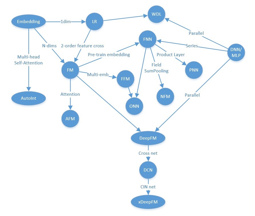
下边这种图连接线会五花八门的，不同人会有不同的理解角度，随便看看就好。

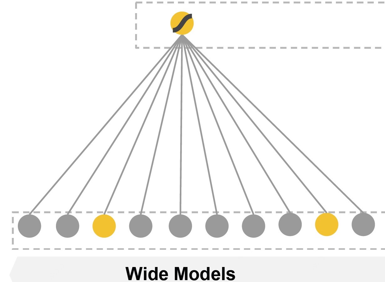
LR

优点：模型简单；时间复杂度低；可大规模并行化；具备一定可解释性；
缺点：依赖大量特征工程；特征交叉困难；未出现的数据泛化性差；

公式：

def lr1(x_id, feature_size):
    """
    x_id: input, feature id;
    feature_size: feature variable space
    """
    embeddings = tf.Variable(tf.random_uniform([feature_size,], -0.1, 0.1))
    b = tf.Variable(tf.random_uniform([1], -1.0, 1.0))
    
    preds = b
    preds += tf.reduce_sum(tf.nn.embedding_lookup(embeddings, x_id))
    
    preds = tf.clip_by_value(tf.sigmoid(preds), 1e-5, 1.0 - (1e-5), name='preds')
    loss = tf.reduce_mean(tf.losses.log_loss(predictions=preds, labels=_Y))

def lr2(x_onehot, feature_size):
    """
    x_onehot: input, onehot(feature_id), size=feature_size;
    feature_size: feature variable space
    """
    embeddings = tf.Variable(tf.random_uniform([feature_size,], -0.1, 0.1))
    b = tf.Variable(tf.random_uniform([1], -1.0, 1.0))
    
    preds = b
    # tf.sparse_tensor_dense_matmul if x_onehot is sparse tensor
    preds += tf.reduce_sum(tf.multiply(embeddings, x_onehot))
    return preds
    

say something:

公式是按照onehot的输入形式给出的，将特征进行onehot展开，输入长度与特征空间长度相同，输入与embedding词表相乘得到对应行的映射权重，即代码 lr2 中实现方式；
但在实际工程中，考虑到输入维度较高、内存以及sparse2dense实现效率的问题，通常是采用代码 lr1 中实现方式，输入为原始id特征，采用embedding_lookup查询到对应行的映射权重。
对于dense feature的处理，先进行embedding_lookup得到embedding，再用dense feature原始数据进行scale, 即(v_ix_i)

embedding dict
标准写法是为每一个field创建一个对应的embedding dict，[emb_dict(space) for space in fieldspacelist]，好处是能隔离开不同field，缺点就是需要维护的向量词表较多；
另一种实现形式就是开辟一个超大的embedding映射空间，将feature_id+namespace组合hash到映射空间内，好处是减少词表维护量，缺点就是耦合了所有field会存在hash冲突导致映射向量的不准；
从经验来看，如果hash方法合适的话，产生hash冲突的概率很小。因此，本文默认采用后者，即模型中只存在一个embedding dict，所有的输入都是经过hash编码后的。

FM: Factorization Machines, 2010

出发点：LR需要手动构造交叉特征；(x_i)=(gender='man' & city='Beijing')，只有两个特征均为 1 时才能更新训练对应的权重；学习不到训练集中未出现的交叉特征，泛化性不好。
优点：可有效处理稀疏场景下的特征学习；具有线行时间复杂度；对训练集中未出现的交叉特征也可进行泛化；
缺点：仅枚举了所有二阶交叉特征，没有考虑高阶；

公式：
D: embedding dim

def fm(x_id, feature_size, dim):
    """
    x_id: input, feature id, tensor_shape=[Batch, field];
    feature_size: feature variable space
    dim: embedding size
    """
    embemdding_matrix = tf.Variable(tf.random_uniform([feature_size, dim], -0.1, 0.1), dtype=tf.float32)
    emb_vec = tf.nn.embedding_lookup(embemdding_matrix, x_id) # Batch*field*Dim (B,F,D)

    square_of_sum = tf.square(tf.reduce_sum(emb_vec, 1))
    sum_of_square = tf.reduce_sum(tf.square(emb_vec), 1)
    
    cross_term = square_of_sum - sum_of_square
    preds = 0.5 * tf.reduce_sum(cross_term, 2)
    return preds

say something:

强制要求所有field的embedding向量的维数，增加了网络复杂度；对连续值特征不友好。

FFM: Field-aware Factorization Machine, 2016

出发点：每个特征xi的隐向量应该有多个，当该特征与不同类型(域field)的特征做交叉时，应该使用对应的隐向量，这样可以做到更精细地刻画交叉特征的权重。所以每个特征应该有和field数量相同的隐向量个数。
优点：引入不同field交叉向量，增加了模型表达能力；
缺点：浅层模型，没有学到高阶交叉特征；

公式：
fj是第j个特征所属的field。

def ffm(x_id, feature_space_list, dim):
    """
    x_id: input, feature_id, tensor_shape=[Batch, field]
    feature_space_list: a list of feature variable space
    dim: embedding size
    """
    def gen_emb_dict(space_size, dim_size):
        return tf.Variable(tf.random_uniform([space_size, dim_size], -0.1, 0.1), dtype=tf.float32)
    embemdding_matrix = [[gen_emb_dict(i, dim) for j in feature_space_list] for i in feature_space_list]

    def feature_embedding(fc_i, fc_j, embedding_dict, input_feature):
        fc_i_embedding = tf.nn.embedding_lookup(embedding_dict[fc_i][fc_j], input_feature) #shape=(B,D)
        return fc_i_embedding
        
    embed_list = []
    for fc_i, fc_j in itertools.combinations(range(len(feature_space_list))):
        i_input = x_id[:,fc_i]
        j_input = x_id[:,fc_j]

        fc_i_embedding = feature_embedding(fc_i, fc_j, embemdding_matrix, i_input)
        fc_j_embedding = feature_embedding(fc_j, fc_i, embemdding_matrix, j_input)

        element_wise_prod = tf.reduce_sum(fc_i_embedding * fc_j_embedding, -1)
        embed_list.append(element_wise_prod)

    ffm_cross = tf.concat(embed_list, axis=1)
    ffm_out = tf.reduce_sum(ffm_cross, -1)

say something:

收益更多的来自扩展了模型参数空间，简单粗暴但有收益，在工业场景落地则对计算资源要求极高。

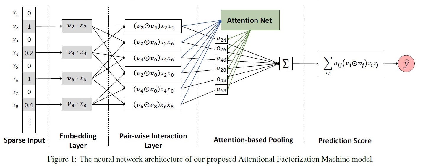
AFM: Attention Factorization Machines, 2017

出发点：FM枚举所有二阶交叉特征，但部分交叉特征与预估目标关联性不大（如广告位尺寸与性别的交叉）。
优点：在FM基础上引入Attention机制，赋予不同交叉特征不同的重要程度；一定程度上增加了模型的可解释性；
缺点：仍是一种浅层模型，没有学到高阶交叉特征

公式：
(igodot) : element-wise

def AFM(x_id, feature_size, dim, attention_factor)
    """
    x_id: input, feature id, shape=[Batch, field]
    feature_size: feature variable space
    dim: embedding size
    attention_factor: dimensionality of the attention network output space.
    """
    field_size = x_id.get_shape().as_list()[1]
    embemdding_matrix = tf.Variable(tf.random_uniform([feature_size, dim], -0.1, 0.1), dtype=tf.float32)
    attention_W = tf.Variable(tf.random_uniform([dim, attention_factor], -0.1, 0.1), dtype=tf.float32)
    attention_b = tf.Variable(tf.random_uniform([attention_factor,], -0.1, 0.1), dtype=tf.float32)
    projection_h = tf.Variable(tf.random_uniform([attention_factor, 1], -0.1, 0.1), dtype=tf.float32)
    projection_p = tf.Variable(tf.random_uniform([embedding_size, 1], -0.1, 0.1), dtype=tf.float32)

    emb_vec = tf.nn.embedding_lookup(embemdding_matrix, x_id) # Batch*field*Dim (B,F,D)
    
    # element_wise, inner_product
    embeds_vec_list = tf.split(emb_vec, field_size, 1) # [(B,1,D)]*F
    row = []; col = []
    import itertools
    for r, c in itertools.combinations(embeds_vec_list, 2):
        row.append(r)
        col.append(c)
    p = tf.concat(row, axis=1)  #pair = (F*F-F)/2, shape(B, pair, D)
    q = tf.concat(col, axis=1)
    inner_product = p * q

    # ###another: element_wise, inner_product
    # inner_product_list = []
    # for i in range(field_size):
    #     for j in range(i+1, field_size):
    #         tmp = tf.multiply(emb_vec[:,i,:], emb_vec[:,j,:])
    #         inner_product_list.append(tmp) # shape=[B,D]
    # inner_product = tf.stack(inner_product_list) # shape=[pair,B,D]
    # inner_product = tf.transpose(inner_product, perm=[1,0,2]) # shape=[B,pair,D]


    attention_temp = tf.nn.relu(tf.tensordot(inner_product, attention_W, axes=(-1, 0)) + attention_b)   
    normalized_att_score = tf.nn.softmax(tf.tensordot(attention_temp, projection_h, axes=(-1, 0)), dim=1)  # shape=[B,pair,1]
    attention_output = tf.reduce_sum(normalized_att_score * inner_product, axis=1)  # shape=[B,D]
    
    afm_out = tf.tensordot([attention_output, projection_p])    # shape=[B,1]
    return afm_out

say something:

AFM是FM的泛化形式，当(p=[1,1,...,1]^T quad and quad alpha_{ij}=1)时，AFM退化成FM模型。

FNN: Factorisation Machine supported Neural Network, 2016

出发点：FM没有考虑高阶交叉特征，DNN具备高阶特征交叉能力。
优点：离线训练FM得到embedding再输入NN，相当于引入先验经验；加速模型的训练和收敛；NN模型节省了学习特征向量的步骤，训练开销低；
缺点：两阶段模型，非endtoend，不利于online learning；预训练embedding受FM模型的限制；只考虑了特征的高阶交叉，没有保留低阶特征信息；

模型：
将FM预训练好的embedding向量直接输入下游DNN

def FNN(x_id, embemdding_matrix, layer_size):
    """
    x_id: input, feature id, shape=[Batch, field]
    embedding_matrix: pretrain FM model embedding vector
    layer_size: a list of DNN layer size, [200,80,1]
    """
    emb_vec = tf.nn.embedding_lookup(embemdding_matrix, x_id) # Batch*field*Dim (B,F,D)
    enc = emb_vec
    for i in layer_size:
        enc = tf.layers.dense(enc, i, activation=tf.nn.leaky_relu)
    return enc

PNN: Product-based Neural Network, 2016

出发点：DNN中特征向量通过简单concat or add都不足以学习到特征之间的依赖关系，因此需要引入更复杂和充分的特征交叉关系的学习。
优点：通过z部分保留了低阶embedding特征信息；通过product layer引入更复杂的特征交叉方式；
缺点：计算时间复杂度相对较高；product函数的实现直接决定了落地可行性；

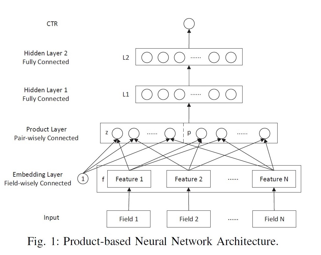
模型:
将每个field的embedding向量输入product layer，在product layer中包含了两部分，一部分是左边的z 直接保留了embedding向量，另一部分右边的p (pair-wise特征交叉)是对应特征之间的product操作。
Product layer：inner product, outer product, kernel product;
对于内积形式的PNN， 两向量相乘的结果为标量，可以直接把各个标量concat拼接成一个大向量，作为MLP的输入。
对于外积形式的PNN， 两向量相乘相当于列向量与行向量进行矩阵相乘，得到结果为一个矩阵。论文简化方案是将各个矩阵进行加和，得到新矩阵拉长成向量后输入MLP。

公式：D is embedding dim; (D_{L1}) is L1 layer size;
IPNN:

P矩阵flatten后就是全连接操作，(W_p=shape[(F*F),D_{L1}])

OPNN:

def PNN(x_id, feature_size, dim)
    """
    x_id: input, feature id, shape=[Batch, field]
    feature_size: feature variable space
    dim: embedding size
    """
    field_size = x_id.get_shape().as_list()[1]
    embemdding_matrix = tf.Variable(tf.random_uniform([feature_size, dim], -0.1, 0.1), dtype=tf.float32)
    emb_vec = tf.nn.embedding_lookup(embemdding_matrix, x_id) # Batch*field*Dim (B,F,D)


    # inner_product
    embeds_vec_list = tf.split(emb_vec, field_size, 1) # [(B,1,D)]*F
    row = []; col = []
    import itertools
    for r, c in itertools.combinations(embeds_vec_list, 2):
        row.append(r)
        col.append(c)
    p = tf.concat(row, axis=1)  #pair = (F*F-F)/2, shape(B, pair, D)
    q = tf.concat(col, axis=1)
    inner_product = p * q   #shape(B, pair, D)
    inner_product = tf.reduce_sum(inner_product, axis=2)

    # outer product
    embedding_sum = tf.reduce_sum(emb_vec,axis=1)
    p = tf.matmul(tf.expand_dims(embedding_sum,2),tf.expand_dims(embedding_sum,1)) # shape=[B,D,D]
    outer_product = tf.layers.flatten(p)
    

    # kernel product
    row = []; col = []
    for i in range(field_size - 1):
        for j in range(i + 1, field_size):
            row.append(i)
            col.append(j)
    # shape=[B,pair,D]
    p = tf.transpose(
        # shape=[pair,B,D]
        tf.gather(
            # shape=[F,B,D]
            tf.transpose(emb_vec, [1, 0, 2]),
            row),
        [1, 0, 2])
    q = tf.transpose(
        tf.gather(
            tf.transpose(emb_vec, [1, 0, 2]),
            col),
        [1, 0, 2])
    num_pairs = len(row)
    p = tf.reshape(p, [-1, num_pairs, dim])
    q = tf.reshape(q, [-1, num_pairs, dim])
    kernel = tf.Variable(tf.random_uniform([dim, num_pairs, dim], -0.1, 0.1), dtype=tf.float32)
    p = tf.expand_dims(p, 1)
    # shape=[B,pair,D]
    kp = tf.multiply(
            # shape=[B,pair,D]
            tf.transpose(
                # shape=[B,D,pair]
                tf.reduce_sum(
                    # shape=[B,D,pair,D]
                    tf.multiply(p, self.kernel),
                    -1),
                [0, 2, 1]),
            q)
    # shape=[B,pair]
    kernel_product = tf.reduce_sum(kp, -1)

公式优化：IPNN通过矩阵分解跳过显示productlayer，通过代数转换直接从embedding到了L1隐层；OPNN直接在productlayer进行优化；
IPNN:

L1层空间复杂度(O(D_{L1}FD+D_{L1}F^2)->O(D_{L1}FD))；时间复杂度(O(D_{L1}FD+D_{L1}F^2)->O(D_{L1}FD+D_{L1}D^2))

OPNN:

L1层时间空间复杂度(O(D_{L1}D^2F^2)->O(D_{L1}DF+D_{L1}D^2))，信息同样损失严重。

def PNN():
    quadratic_output = []

    if use_inner:
        weights['inner'] = tf.Variable(tf.random_normal([L1_size,field_size],0.0,0.01))
        for i in range(L1_size):
            theta = tf.multiply(emb_vec,tf.reshape(weights['inner'][i],(1,-1,1))) # shape=(B,F,D)
            quadratic_output.append(tf.reshape(tf.norm(tf.reduce_sum(theta,axis=1),axis=1),shape=(-1,1))) # shape=(B,1)
    elif use_outer:
        weights['outer'] = tf.Variable(tf.random_normal([L1_size, field_size,field_size], 0.0, 0.01))
        embedding_sum = tf.reduce_sum(emb_vec,axis=1)
        p = tf.matmul(tf.expand_dims(embedding_sum,2),tf.expand_dims(embedding_sum,1)) # shape=(B,D,D)
        for i in range(L1_size):
            theta = tf.multiply(p,tf.expand_dims(self.weights['outer'][i],0)) # shape=(B,D,D)
            quadratic_output.append(tf.reshape(tf.reduce_sum(theta,axis=[1,2]),shape=(-1,1))) # shape=(B,1)
    
    lp = tf.concat(quadratic_output,axis=1)

say something:

这实际是一篇会转刊的文章，网上能搜到两个版本，一个是2016年的ICDM，一个是2018年的TOIS，在转刊时不能完全相同，因此文章把outer product部分替换成了kernel product；kernel的设计更复杂了，但还是outer的泛化，把kernel看成tf.ones()就会退化到outer,

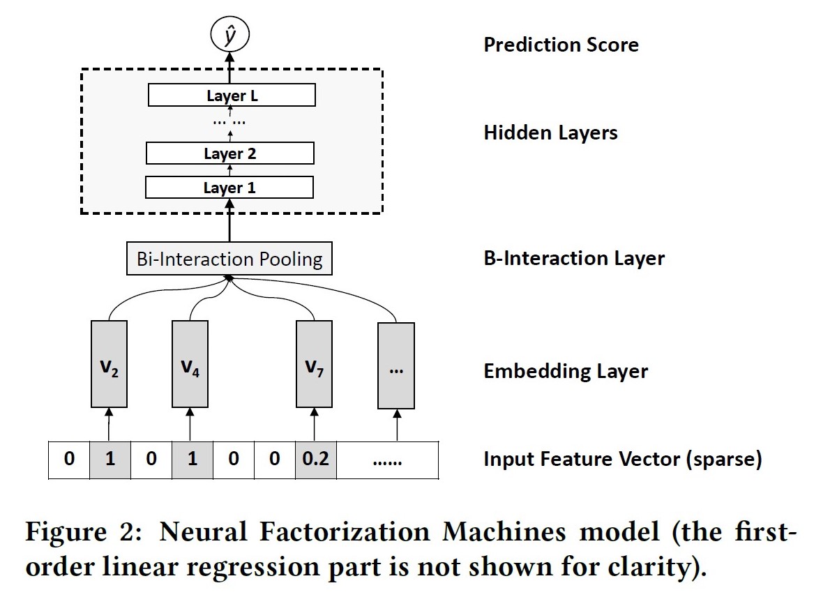
NFM: Neural Factorization Machines, 2017

出发点：FM枚举所有二阶交叉特征，没有高阶交叉特征
优点：相比于concat操作，NFM在low level进行interaction可以提高模型的表达能力；具备一定高阶特征交叉能力；Bi-Interaction Pooling的交叉具备线性复杂度；
缺点：直接进行sum pooling操作会损失信息，可参考AFM的操作；

公式：
Bi-Interaction操作，名字挺高大上，其实就是一个计算FM的过程，将所有二阶交叉结果向量在field维度进行sum pooling后再送入NN进行训练。

def bi_interaction(x_id, feature_size, dim):
    """
    x_id: input, feature id, tensor_shape=[Batch, field];
    feature_size: feature variable space
    dim: embedding size
    """
    embemdding_matrix = tf.Variable(tf.random_uniform([feature_size, dim], -0.1, 0.1), dtype=tf.float32)
    emb_vec = tf.nn.embedding_lookup(embemdding_matrix, x_id) # Batch*field*Dim (B,F,D)

    square_of_sum = tf.square(tf.reduce_sum(emb_vec, 1))
    sum_of_square = tf.reduce_sum(tf.square(emb_vec), 1)
    
    cross_term = 0.5 * (square_of_sum - sum_of_square)
    return cross_term

say something:

当NN的全连接都是恒等变换且最后一层参数全为1， NFM就退化为FM。NFM是FM的推广，延迟了FM的实现过程，在其中加入更多非线形运算。

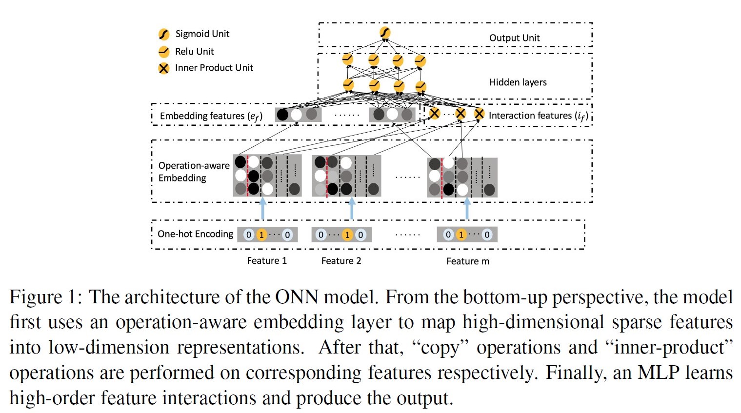
ONN: Operation-aware Neural Network, 2019

出发点：不同的特征交叉操作，应该使用不同的embedding，相同的embedding在不同操作间会相互影响而最终限制了模型的表达。
优点：引入Operation-aware，增加了模型表达能力；同时包含了特征一阶信息和高阶交叉信息；
缺点：模型复杂度高；每个feature对应多个embedding结果；

模型：
一个feature对应多个embedding，第一列的embedding是feature本身的信息，从第二列开始往后是当前特征与第n个特征交叉所使用的embedding。

def ONN(x_id, feature_space_list, dim):
    """
    x_id: input, feature_id, tensor_shape=[Batch, field]
    feature_space_list: a list of feature variable space
    dim: embedding size
    """
    def gen_emb_dict(space_size, dim_size):
        return tf.Variable(tf.random_uniform([space_size, dim_size], -0.1, 0.1), dtype=tf.float32)
    embemdding_matrix = [[gen_emb_dict(i, dim) for j in feature_space_list] for i in feature_space_list]

    def feature_embedding(fc_i, fc_j, embedding_dict, input_feature):
        fc_i_embedding = tf.nn.embedding_lookup(embedding_dict[fc_i][fc_j], input_feature) #shape=(B,D)
        return fc_i_embedding
        
    embed_list = []
    for fc_i, fc_j in itertools.combinations(range(len(feature_space_list))):
        i_input = x_id[:,fc_i]
        j_input = x_id[:,fc_j]

        fc_i_embedding = feature_embedding(fc_i, fc_j, embemdding_matrix, i_input)
        fc_j_embedding = feature_embedding(fc_j, fc_i, embemdding_matrix, j_input)

        element_wise_prod = tf.reduce_sum(fc_i_embedding * fc_j_embedding, -1)
        embed_list.append(element_wise_prod)

    onn_cross = tf.concat(embed_list, axis=1)
    onn_out = DNN(onn_cross)

say something:

模型结构并没有太惊艳，积木拼接FFM+NN=ONN。
FFM/AFM/ONN通过引入额外的信息来区分不同field间的交叉应该具备不同的信息表达和重要性。

WDL: Wide and Deep Learning, 2016

出发点：首次使用双路并行的结构，结合Wide线行模型的记忆性(memorization)和Deep深度模型的泛化性(generalization)来对用户行为信息进行学习建模。
优点：Wide&Deep互补，Deep弥补Memorization层泛化性不足的问题；wide&deep joint training可减少wide部分的model size(即只需要少数的交叉特征)；可以同时学习低阶特征交叉wide和高阶特征交叉deep;
缺点：仍需要手动设计交叉特征；

公式：

def wdl(x_id, feature_size):
    embeddings = tf.Variable(tf.random_uniform([feature_size,], -0.1, 0.1))
    b = tf.Variable(tf.random_uniform([1], -1.0, 1.0))
    inp = tf.nn.embedding_lookup(embeddings, x_id)

    lr = tf.reduce_sum(inp)
    nn = DNN(inp)
    preds = b+lr+nn

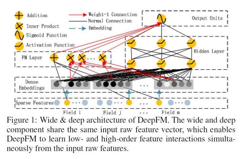
DeepFM: Deep Factorization Machines, 2017

出发点：FM基础上引入NN隐式高阶交叉信息；
优点：模型同时学习低阶和高阶特征能力；共享embedding，共享参数信息表达；
缺点：DNN部分对于高阶特征的学习仍然是隐式的；

公式：

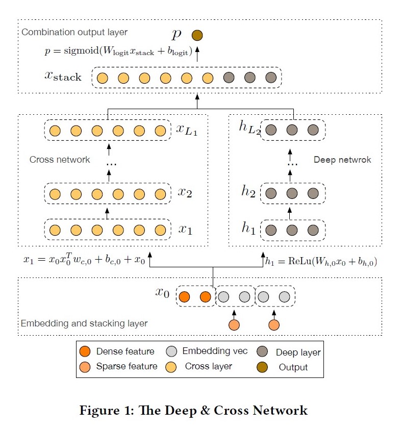
DCN: Deep and Cross Network, 2017

出发点：DNN的高阶交叉学习能力是隐式的，wide侧的交叉组合特征主要是人工特征工程或暴力搜索（exhaustive searching），因此提出cross net可以显示的学习有限阶（bounded degrees）的特征交叉；
优点：具备显示高阶特征交叉能力；结合ResNet思想，将原始信息在crossnet中跳跃传递；crossNet结构简单，节省内存计算高效；
缺点：CrossNet在进行交叉时采用bit-wise方式，直接concat淹没了field的概念；每层的输出都是输入向量(x_0)的标量倍（不是线行倍），这种形式在一定程度上限制了模型的表达能力；

公式：

证明：输出都是输入向量(x_0)的标量倍（忽略偏置项）

def cross_layer(x0, x, name):
    """
    x0,x: input tensor, shape=(B,N)
    """
    with tf.variable_scope(name):
        input_dim = x0.get_shape().as_list()[1]
        w = tf.get_variable("weight", [input_dim], initializer=tf.truncated_normal_initializer(stddev=0.01))
        b = tf.get_variable("bias", [input_dim], initializer=tf.truncated_normal_initializer(stddev=0.01))
        xb = tf.tensordot(tf.reshape(x, [-1, 1, input_dim]), w, 1)
        return x0 * xb + b + x

def build_cross_layers(x_id, feature_size, dim, num_cross_layers, hidden_size_lst):
    embemdding_matrix = tf.Variable(tf.random_uniform([feature_size, dim], -0.1, 0.1), dtype=tf.float32)
    emb_vec = tf.nn.embedding_lookup(embemdding_matrix, x_id) # Batch*field*Dim (B,F,D)
    B = emb_vec.get_shape().as_list()[0]
    x0 = tf.reshape(emb_vec, [B,-1]) # shape=(B,N), N=F*D

    ## cross layer
    x = x0
    for i in range(num_cross_layers):
        x = cross_layer2(x0, x, 'cross_{}'.format(i))
    cross_layer = x

    ## deep layer
    net = x0
    for units in hidden_size_lst:
        net = tf.layers.dense(net, units=units, activation=tf.nn.relu)
    deep_layer = net

    out = tf.concat([cross_layer, deep_layer], 1)

say something:

在cross_layer实现的时候，先计算了结果为标量的(x_l^Tw)，而非按照公式从左到右计算，主要是考虑到临时存储内存空间的大小，(x_0x_l^T)这一个操作需要的内存就是(batch\_size*(filed*dim)*(filed*dim)*(4or8))，这仅仅是一层的操作，矩阵与向量相乘也是非常消耗计算资源的，在企业场景中这是难以接受的((ifquad filed*dim=1k, batch=1k, float, one\_layer\_memory=4G))，因此利用矩阵乘法的结合律，先计算(x_l^Tw)得到标量，几乎不占存储空间，再与权重向量相乘。
这多说一句性能，可能在离线实验时并没有关注模型性能问题，主要以实现功能为主，但后期有效果需要上线时就要考虑代码实现方式的问题了，曾经有一次架构人员忙了半个月才优化下去20%的耗时，我从模型代码实现方式这块优化50%的耗时，并不是后者多牛逼（毕竟最初版本的烂代码也是自己写的），只是大家站在不同的角度去解决问题，很多时候性能问题在离线验证中是最容易被忽略的。

xDeepFM: eXtreme Deep Factorization Machine, 2018

出发点：解决DCN的输出被限制在特征形式上，与DeepFM相比和DCN是近亲;
优点：同时学习到显示的高阶特征交叉(CIN)与隐式的高阶特征交叉(DNN)；在交叉特征CIN的学习上采用vector-wise的交叉；
缺点：CIN的时间复杂度较高；CIN的sum pooling会损失信息；

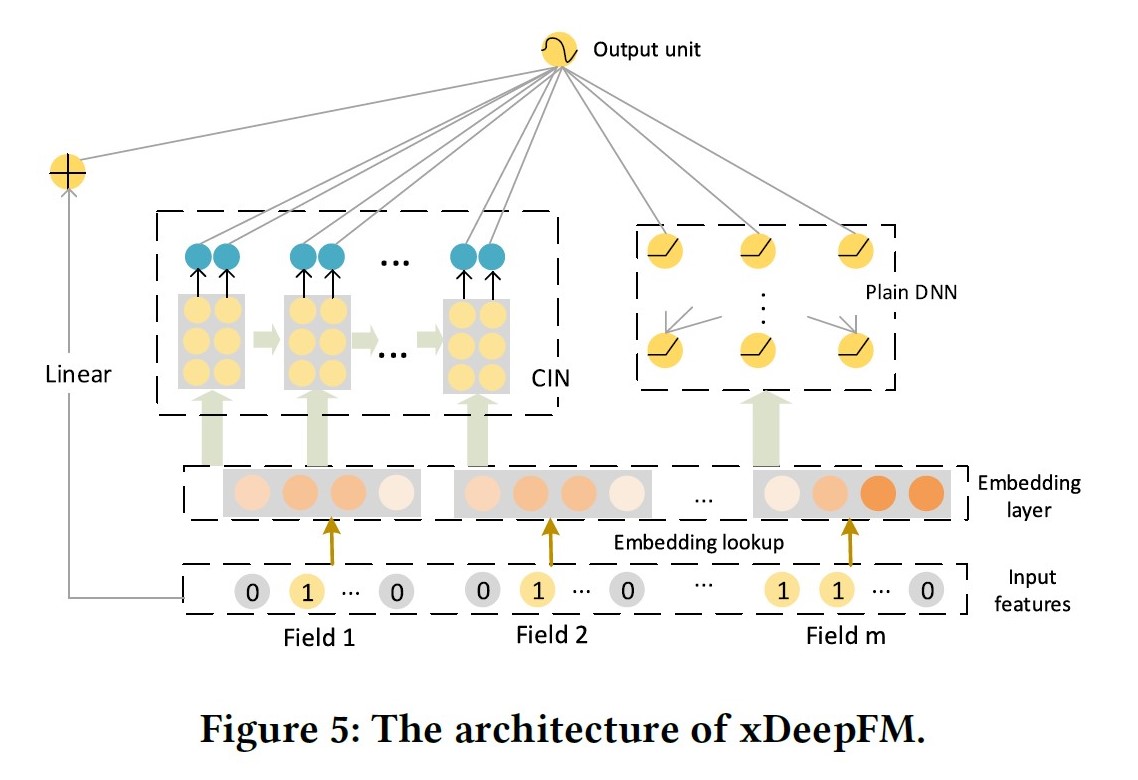
模型分为三部分：

• Linear Part: 捕获线性特征；
• DNN Part: 隐式的、bit-wise的学习高阶交叉特征；
• CIN Part: 压缩交互网络，显示的、vector-wise的学习高阶交叉特征；

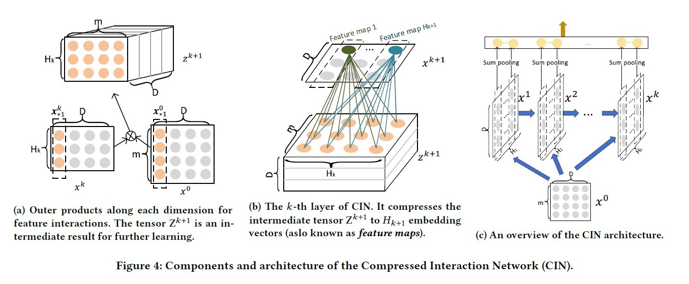
CIN结构：
令(X^kin R^{H_k*D})表示第(k)层的输出，其中(H_k)表示第(k)层的vector个数，vecor维度始终为(D) ，保持和输入层一致。具体地，第(k)层每个vector的计算方式为：

其中W^{k,h}表示第(k)层的第(h)个vector的权重矩阵， (circ)表示Hadamard乘积，即逐元素乘，例如(<a1,b1,c1>circ <a2,b2,c2>=<a1*a2,b1*b2,c1*c2>)。

取前一层(X^{k-1}in R^{H_{k-1}*D})中的(H_{k-1})个vector，与输入层(X^0in R^{m*D})中的m个vector，进行两两Hadamard乘积(外积)运算，得到(H_{k-1}*m)个vector，然后加权求和。
第k层的不同vector区别在于，对这(H_{k-1}*m)个vector求和的权重矩阵不同。权重(W^{k,i}in R^{H_{k-1}*m}顺着tensor维度D逐层相乘相加，得到k层第i个向量，)H_k(即对应有多少个不同的权重矩阵)W^k$ , 是一个可以调整的超参。
将外积结果看成是三维矩阵(m*H_k*D),不同权重在维度D方向上加权求和，可看作是在(m*H_k)整个平面上的卷积操作。

def _build_extreme_FM(hparams, nn_input, field_num, dim, cross_layer_sizes):
    hidden_nn_layers = []
    field_nums = []
    final_len = 0
    nn_input = tf.reshape(nn_input, shape=[-1, field_num, dim])  # shape=(B F0 D)
    field_nums.append(field_num) 
    hidden_nn_layers.append(nn_input)
    final_result = []

    split_tensor0 = tf.split(hidden_nn_layers[0], dim * [1], 2) # [shape=(B F0 1)]*D
    with tf.variable_scope("exfm_part", initializer=self.initializer) as scope:
        for idx, layer_size in enumerate(cross_layer_sizes):
    
            split_tensor = tf.split(hidden_nn_layers[-1], dim * [1], 2) # [shape=(B Fi 1)]*D
            dot_result_m = tf.matmul(split_tensor0, split_tensor, transpose_b=True) # shape=(D B F0 Fi)
            dot_result_o = tf.reshape(dot_result_m, shape=[dim, -1, field_nums[0]*field_nums[-1]])
            dot_result = tf.transpose(dot_result_o, perm=[1, 0, 2]) # shape=(B D F0*Fi) 

            filters = tf.get_variable(name="f_"+str(idx),
                                 shape=[1, field_nums[-1]*field_nums[0], layer_size], # shape=(1 F0*Fi F{i+1})
                                 dtype=tf.float32)  

            curr_out = tf.nn.conv1d(dot_result, filters=filters, stride=1, padding='VALID') # shape=(B D F{i+1})
            curr_out = tf.nn.relu(curr_out)
            curr_out = tf.transpose(curr_out, perm=[0, 2, 1]) # shape=(B Fi+1 D)

            direct_connect = curr_out
            next_hidden = curr_out
            final_len += layer_size
            field_nums.append(int(layer_size))

            final_result.append(direct_connect)
            hidden_nn_layers.append(next_hidden)

        result = tf.concat(final_result, axis=1)
        result = tf.reduce_sum(result, -1)

        w_nn_output = tf.get_variable(name='w_nn_output',
                                      shape=[final_len, 1],
                                      dtype=tf.float32)
        b_nn_output = tf.get_variable(name='b_nn_output',
                                      shape=[1],
                                      dtype=tf.float32,
                                      initializer=tf.zeros_initializer())

        exFM_out = tf.nn.xw_plus_b(result, w_nn_output, b_nn_output)

        return exFM_out

say something:

如果CIN只有一层，(H_1=m, W^1=1),则sum pooling的输出结果就是一系列两两向量内积之和，是标准FM。
复杂度分析，假设CIN和DNN每层向量/神经元个数都为H，网络深度为T。CIN的参数空间复杂度为(O(mTH^2)) ，普通的DNN为(O(mDH+TH^2))，CIN的空间复杂度与输入维度D无关。CIN的时间复杂度为(O(mH^2DT)) ，而DNN为(O(mDH+TH^2))，时间复杂度会是CIN的一个主要痛点。
DCN的残差项保证了特征的1～l+1特征都有，而CIN中去除了残差项，虽然更快了，但是相当于丢弃了1～l阶特征的组合结果。

AutoInt: Automatic Feature Interaction Learning

出发点：使用multi-head self attention(Transformer里的那个) 机制来进行自动特征交叉学习，以提升CTR预测任务的精度；
优点：可显示的以vector-wise的方式学习有限阶特征交叉信息；

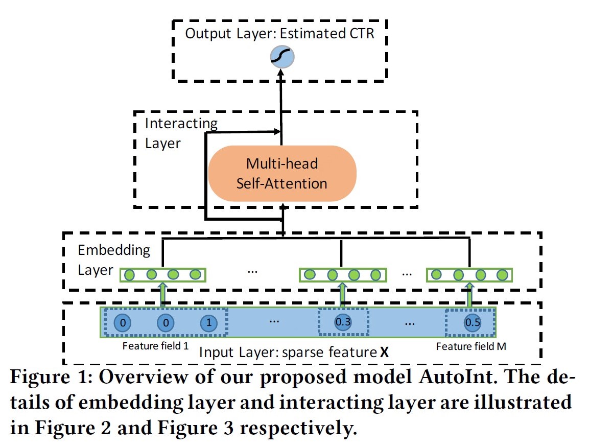
模型：
AutoInt直接采用了单路的模型结构，将原始特征embedding后直接进行Self-attention操作，将输入与输出连接做残差ResNet，多层堆叠后输出。论文中给出了AutoInt+DNN的双路模型实验AutoInt+。

文章里拆分的公式看着太费劲，还是Transformer里的刚易懂。

def multihead_attention(queries, keys, values,
                        num_units=None,
                        num_heads=1,
                        dropout_keep_prob=1,
                        is_training=True,
                        has_residual=True):
    if num_units is None:
        num_units = queries.get_shape().as_list[-1]

    # Linear projections
    Q = tf.layers.dense(queries, num_units, activation=tf.nn.relu)
    K = tf.layers.dense(keys, num_units, activation=tf.nn.relu)
    V = tf.layers.dense(values, num_units, activation=tf.nn.relu)

    Q_ = tf.concat(tf.split(Q, num_heads, axis=2), axis=0)
    K_ = tf.concat(tf.split(K, num_heads, axis=2), axis=0)
    V_ = tf.concat(tf.split(V, num_heads, axis=2), axis=0)

    QK = tf.matmul(Q_, tf.transpose(K_, [0, 2, 1]))
    weights = QK / (K_.get_shape().as_list()[-1] ** 0.5)
    weights = tf.nn.softmax(weights)
    weights = tf.layers.dropout(weights, rate=1-dropout_keep_prob,
                                        training=tf.convert_to_tensor(is_training))

    # Weighted sum
    outputs = tf.matmul(weights, V_)

    # Restore shape
    outputs = tf.concat(tf.split(outputs, num_heads, axis=0), axis=2)

    # Residual connection
    if has_residual:
        V_res = tf.layers.dense(values, num_units, activation=tf.nn.relu)
        outputs += V_res

    outputs = tf.nn.relu(outputs)
    # Normalize
    outputs = normalize(outputs)
        
    return outputs

def AutoInt(x_id, feature_size, dim, blocks):
    field_size = x_id.get_shape().as_list()[1]
    embemdding_matrix = tf.Variable(tf.random_uniform([feature_size, dim], -0.1, 0.1), dtype=tf.float32)
    emb_vec = tf.nn.embedding_lookup(embemdding_matrix, x_id) # Batch*field*Dim (B,F,D)

    for i in range(blocks):
        emb_vec = multihead_attention(queries=emb_vec, keys=emb_vec, values=emb_vec)
    flat = tf.reshape(emb_vec, shape=[-1, dim * field_size])
    out = tf.layers.dense(flat, 1, activation=None)

say something:

如果看过"Attenion is all you need"论文的话，这个工作很快就能看完并理解，连作者开源的代码都是直接从Transformer的gitcode中扒下来的。工作虽然是已有知识迁移到ctr领域，但仍是很好的创新，模型结构清晰简洁。
墙裂案例https://www.github.com/kyubyong/transformer 这个代码。

overview:
https://blog.csdn.net/han_xiaoyang/article/details/81031961
https://zhuanlan.zhihu.com/p/104307718
PNN: https://zhuanlan.zhihu.com/p/56651241
ONN: https://cloud.tencent.com/developer/news/456076
DCN: http://xudongyang.coding.me/dcn/
ffm: https://tech.meituan.com/2016/03/03/deep-understanding-of-ffm-principles-and-practices.html
autoint: https://zhuanlan.zhihu.com/p/60185134
xdeepFM:
https://www.jianshu.com/p/b4128bc79df0
http://www.shataowei.com/2019/12/17/xDeepFM架构理解及实现/
http://xudongyang.coding.me/xdeepfm/
https://zhuanlan.zhihu.com/p/57162373
https://blog.csdn.net/DaVinciL/article/details/81359245