摘要:
matlab中提供了核平滑密度估计函数ksdensity:[f,xi]=ksdensity返回矢量或两列矩阵x中的样本数据的概率密度估计f。该估计基于高斯核函数,并且在等间隔的点xi处进行评估,覆盖x中的数据范围。ksdensity估计单变量数据的100点密度,或双变量数据的900点密度。ksdensity适用于连续分布的样本。也可以指定评估点:[f,xi]=ksdensityspecifiespointstoevaluatef.Here,xiandptscontainidenticalvalues。
matlab中提供了核平滑密度估计函数ksdensity(x):
[f, xi] = ksdensity(x)
返回矢量或两列矩阵x中的样本数据的概率密度估计f。 该估计基于高斯核函数,并且在等间隔的点xi处进行评估,覆盖x中的数据范围。
ksdensity估计单变量数据的100点密度,或双变量数据的900点密度。
ksdensity适用于连续分布的样本。
也可以指定评估点:
[specifies points (f,xi] = ksdensity(x,pts)pts) to evaluatef. Here,xiandptscontain identical values。
核密度估计方法:

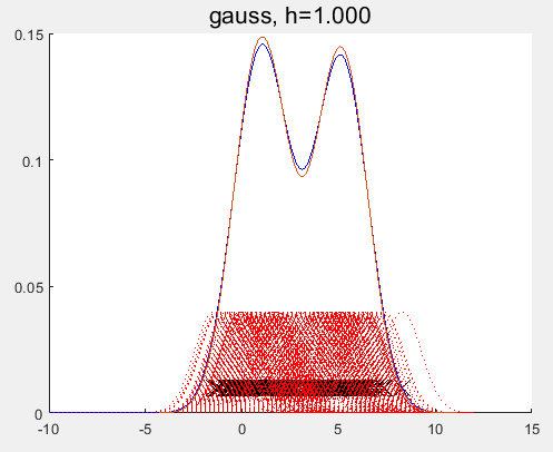
代码实现,对比:
clear all;
clc;
n=100;
% 生成一些正态分布的随机数
x=normrnd(0,1,1,n);
minx = min(x);
maxx = max(x);
dx = (maxx-minx)/n;
x1 = minx:dx:maxx-dx;
h=0.5;
f=zeros(1,n);
for j = 1:n
for i=1:n
f(j)=f(j)+exp(-(x1(j)-x(i))^2/2/h^2)/sqrt(2*pi);
end
f(j)=f(j)/n/h;
end
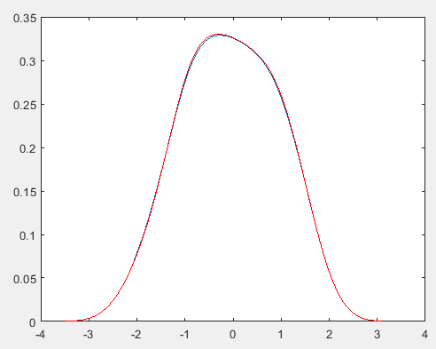
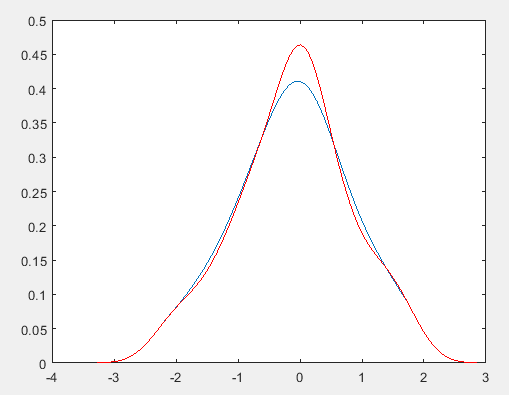
plot(x1,f);
%用系统函数计算比较
[f2,x2] = ksdensity(x);
hold on;
plot(x2,f2,'r'); %红色为参考
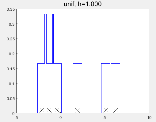
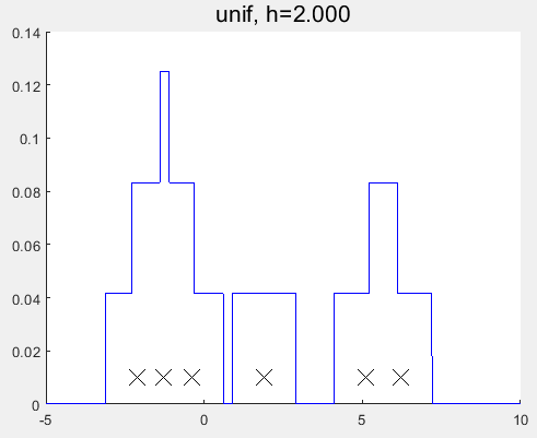
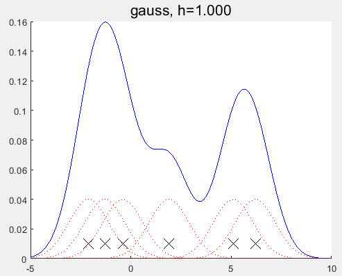
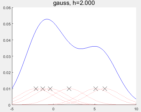
PRML上核密度估计(parzen窗密度估计)的实现:
%% Demonstrate a non-parametric (parzen) density estimator in 1D
%%
% This file is from pmtk3.googlecode.com
function parzenWindowDemo2
% setSeed(2);
%[data, f] = generateData;
%  http://en.wikipedia.org/wiki/Kernel_density_estimation
data = [-2.1 -1.3 -0.4 1.9 5.1 6.2]';
f = @(x) 0;
n = numel(data);
domain = -5:0.001:10;
kernels = {'gauss', 'unif'};
for kk=1:2
  kernel = kernels{kk};
  switch kernel
    case 'gauss', hvals = [1, 2];
    case 'unif', hvals = [1, 2];
  end
  for i=1:numel(hvals)
    h = hvals(i);
    figure;
    hold on
    handle=plot(data, 0.01*ones(1,n), 'x', 'markersize', 14);
    set(handle,'markersize',14,'color','k');
    g = kernelize(h, kernel, data);
    plot(domain,g(domain'),'-b');
    if strcmp(kernel, 'gauss')
      for j=1:n
        k = @(x) (1/h)*gaussProb(x,data(j),h^2);
        plot(domain, 0.1*k(domain'), ':r');
      end
    end
    title(sprintf('%s, h=%5.3f', kernel, h), 'fontsize', 16);
    %printPmtkFigure(sprintf('parzen-%s-%d', kernel, h));
  end
  %placeFigures('nrows',3,'ncols',1,'square',false);
end
end
function [data, f] = generateData
mix = [0.35,0.65];
sigma = [0.015,0.01];
mu = [0.25,0.75];
n = 50;
%% The true function, we are trying to recover
f = @(x)mix(1)*gaussProb(x, mu(1), sigma(1)) + mix(2)*gaussProb(x, mu(2), sigma(2));
%Generate data from a mixture of gaussians.
model1 = struct('mu', mu(1), 'Sigma', sigma(1));
model2 = struct('mu', mu(2), 'Sigma', sigma(2));
pdf1 = @(n)gaussSample(model1, n);
pdf2 = @(n)gaussSample(model2, n);
data = rand(n,1);
nmix1 = data <= mix(1);
data(nmix1) = pdf1(sum(nmix1));
data(~nmix1) = pdf2(sum(~nmix1));
end
function g = kernelize(h,kernel,data)
%Use one gaussian kernel per data point with smoothing parameter h.
n = size(data,1);
g = @(x)0;
%unif = @(x, a, b)exp(uniformLogprob(structure(a, b), x));
for i=1:n
  switch kernel
    case 'gauss', g = @(x)g(x) + (1/(h*n))*gaussProb(x,data(i),h^2);
    %case 'unif', g = @(x)g(x) + (1/n)*unif(x,data(i)-h/2, data(i)+h/2);
    case 'unif', g = @(x)g(x) + (1/(h*n))*unifpdf(x,data(i)-h/2, data(i)+h/2);
  end
end
end
function setupFig(h)
figure;
hold on;
axis([0,1,0,5]);
set(gca,'XTick',0:0.5:1,'YTick',[0,5],'box','on','FontSize',16);
title(['h = ',num2str(h)]);
scrsz = get(0,'ScreenSize');
left =  20;   right = 20;
lower = 50;   upper = 125;
width = scrsz(3)-left-right;
height = (scrsz(4)-lower-upper)/3;
set(gcf,'Position',[left,scrsz(4)/2,width, height]);
end
function p = gaussProb(X, mu, Sigma)
% Multivariate Gaussian distribution, pdf
% X(i,:) is i'th case
% *** In the univariate case, Sigma is the variance, not the standard
% deviation! ***
% This file is from pmtk3.googlecode.com
d = size(Sigma, 2);
X  = reshape(X, [], d);  % make sure X is n-by-d and not d-by-n
X = bsxfun(@minus, X, rowvec(mu));
logp = -0.5*sum((X/(Sigma)).*X, 2);
logZ = (d/2)*log(2*pi) + 0.5*logdet(Sigma);
logp = logp - logZ;
p = exp(logp);
end
function x = rowvec(x)
% Reshape a matrix into a row vector
% Return x as a row vector. This function is useful when a function returns a
% column vector or matrix and you want to immediately reshape it in a functional
% way. Suppose f(a,b,c) returns a column vector, matlab will not let you write
% f(a,b,c)(:)' - you would have to first store the result. With this function you
% can write rowvec(f(a,b,c)) and be assured that the result is a row vector.
% This file is from pmtk3.googlecode.com
    x = x(:)';
end
function y = logdet(A)
% Compute log(det(A)) where A is positive-definite
% This is faster and more stable than using log(det(A)).
%
%PMTKauthor Tom Minka
% (c) Microsoft Corporation. All rights reserved.
% This file is from pmtk3.googlecode.com
try
    U = chol(A);
    y = 2*sum(log(diag(U)));
catch % #ok
    y = 0;
    warning('logdet:posdef', 'Matrix is not positive definite');
end
end
对比发现与MATLAB自带的函数的估计结果仍有一定的差异?

参考: